MAC/GMC 4

MAC/GMC 4.0 User’s Manual

Volume 2:

Keywords Manual

Brett A. Bednarcyk

Steven M. Arnold

Table of Contents............................................................................................................................... 1

Introduction....................................................................................................................................... 2

Current Capabilities and What’s New in MAC/GMC 4.0................................................................... 3

Format of this Manual.................................................................................................................. 6

Getting Started................................................................................................................................... 7

Distributed Files.......................................................................................................................... 7

Executing MAC/GMC 4.0 Problems................................................................................................ 7

Using User-Defined Subroutines with MAC/GMC 4.0...................................................................... 9

Format of the MAC/GMC 4.0 Input File........................................................................................ 10

Section 1 : Flag-Type Keywords......................................................................................................... 12

*CHECK: Check input file for errors................................................................................................ 13

*CONDUCTIVITY: Effective thermal conductivities.......................................................................... 14

*ELECTROMAG: Electromagnetic analysis....................................................................................... 16

Section 2 : Material Keywords............................................................................................................ 18

*MDBPATH: External material database file & location..................................................................... 19

*CONSTITUENTS: Constituent (subcell) materials........................................................................... 21

Section 3 : Analysis Type and Architecture Keywords.......................................................................... 45

*RUC: Repeating unit cell analysis and architecture........................................................................ 48

*LAMINATE: Laminate analysis and architecture............................................................................ 60

Section 4 : Loading Keywords............................................................................................................ 64

*MECH: Applied mechanical loading............................................................................................... 66

*THERM: Applied thermal loading................................................................................................... 70

*SOLVER: Time integration........................................................................................................... 72

*SURF: Yield Surface Analysis....................................................................................................... 76

Section 5 : Damage and Failure Keywords.......................................................................................... 79

*ALLOWABLES: Estimated elastic allowables.................................................................................. 80

*FAILURE_SUBCELL: Subcell static failure.................................................................................... 83

*FAILURE_CELL: Repeating unit cell static failure......................................................................... 86

*DAMAGE: Fatigue damage analysis............................................................................................... 88

*DEBOND: Fiber-matrix interfacial debonding.................................................................................. 94

*CURTIN: Curtin effective fiber breakage model............................................................................. 98

Section 6 : Results and Data Output Keywords................................................................................. 100

*PRINT: Overall print output level for output file.......................................................................... 101

*XYPLOT: X-Y plot output........................................................................................................... 102

*PATRAN: PATRAN post-processing data output........................................................................... 108

*MATLAB: MATLAB post-processing data output........................................................................... 110

Section 7 : End of File Keyword....................................................................................................... 112

*END: End of input file................................................................................................................ 113

References..................................................................................................................................... 114

Appendix........................................................................................................................................ 115

User-Defined Constituent Material Constitutive Model File (usrmat.F90)...................................... 116

User-Defined Stiffness Matrix Determination File (usrformde.F90).............................................. 121

User-Defined Material Property Determination File (usrfun.F90)................................................. 123

Sample external material database file.......................................................................................... 129

MATLAB source files for generation of fringe plots (stress.m, strain.m, epsp.m).................. 130

Index............................................................................................................................................. 147

Introduction

This document is the second volume in the three volume set of User’s Manuals for the Micromechanics Analysis Code with Generalized Method of Cells Version 4.0 (MAC/GMC 4.0). Volume 1 is the Theory Manual, this document is the Keywords Manual, and Volume 3 is the Example Problem Manual.

MAC/GMC 4.0 is a computer code developed at NASA Glenn Research Center that analyzes the thermo-inelastic behavior of composite materials and laminates. The code is based on the micromechanics theory known as the generalized method of cells (GMC). GMC models the response of composite materials using a doubly or triply periodic repeating unit cell (RUC), which is composed of a number of subcells (see Figure 3.1 and Figure 3.2). By placing distinct constituent materials within the subcells, a heterogeneous (composite) material can be modeled, provided an RUC can be identified in the material’s micro scale architecture. The main advantages of GMC over other micromechanics theories and approaches are: 1) its fully multi-axial formulation, 2) the availability of local (constituent level) stress and strain fields, and 3) its computational efficiency. The availability of the local fields makes the method attractive in situations where more detailed composite analysis, beyond simple determination of effective thermo-elastic properties, is necessary. In such situations, when matrix inelasticity, constituent damage or failure, or fiber-matrix debonding is important, the availability of the local fields is critical in order to account for these effects appropriately. It is the purpose of the MAC/GMC 4.0 code to provide a convenient and user-friendly “package” for the GMC theories, in addition to providing significant added value through a library of inelastic constitutive models, repeating unit cells, thermo-mechanical and yield surface loading options, failure and damage analysis capabilities, and results generation options.

The original method of cells (which allowed only four subcells) was developed by Aboudi (1989, 1991), the doubly periodic version of GMC by Paley and Aboudi (1992), and the triply periodic version of GMC by Aboudi (1995). The actual GMC theories implemented within MAC/GMC 4.0 were reformulated for maximum computational efficiency by Pindera and Bednarcyk (1999) and Bednarcyk and Pindera (2000). A recent advancement in the GMC technology has significantly improved the local accuracy of the doubly periodic version of the model. This new micromechanics theory, called the high-fidelity generalized method of cells (HFGMC), developed by Aboudi et al. (2001, 2002), has also been implemented with MAC/GMC 4.0.

As mentioned, MAC/GMC 4.0 is also capable of analyzing composite laminates. The composite laminate analysis capabilities also rely on the GMC composite material model. The doubly and triply periodic versions of GMC function within the context of classical lamination theory (Jones, 1975; Herakovich, 1998) to model the ply level composite material. Thus, the code can analyze the thermo-inelastic behavior of arbitrary laminate configurations.

Finally, a new thermo-electro-magnetic version of GMC that is capable of modeling so-called “smart” composites has been implemented within MAC/GMC 4.0. The implementation also enables the analysis of smart composite laminates. This specific form of the thermo-electro-magnetic GMC was developed by Bednarcyk (2002) based on the work of Aboudi (2000).

Current Capabilities and What’s New in MAC/GMC 4.0

The current capabilities of MAC/GMC are listed below, with new or improved features in this version highlighted in bold blue type. The superscripts refer to the enumerated details regarding these new features given after the list.

Current Capabilities

· Usability

Intuitive ASCII user interface¹

A graphical user interface (GUI) for MAC/GMC 4.0 will be available in March 2002

Computer resource management²

- Dynamic memory allocation

- Static problem size limitations removed

- Improved efficiency of solution for laminate analysis and large problems

43 new example problems are described in the MAC/GMC 4.0 Example Problem Manual and are distributed with the code

· Material Constitutive Models⁵

Elastic: isotropic, transversely isotropic, completely anisotropic

Inelastic: Bodner-Partom, Robinson, isotropic GVIPS, transversely isotropic GVIPS, multimechanism GVIPS, SMA, incremental plasticity, Freed-Walker

User-defined: user-defined constitutive model subroutine (usrmat.F90)

· Library of Material Properties

Expanded internal material property library

Temperature-dependent or temperature-independent properties specified in input file

User-defined subroutine (usrfun.F90) for calculating material properties as a function of temperature or other variable

External material property database file⁶

· Micromechanics Analysis Models

Doubly periodic generalized method of cells

Triply periodic generalized method of cells

Doubly Periodic High-Fidelity Generalized Method of Cells (HFGMC)⁴

· Library of Doubly and Triply Periodic Repeating Unit Cell Architectures

· Laminate Analysis Model (Classical Lamination Theory)

Monolithic layers

Doubly periodic composite layers

Triply periodic composite layers⁷

Improved interoperability (doubly and triply periodic layers in the same laminate)⁷

· Smart Material Analysis Capabilities

Shape memory alloy (SMA) model⁵

Fully coupled thermo-electro-magneto-elasto-plastic analysis³

- Constituent material (arbitrary poling direction)

- Composite

- Laminate

· Library of Applied Loading History Options

Thermal, uniaxial, biaxial, general (arbitrary) loading, thermo-mechanical

Curvature and moment loading for laminate

Electromagnetic loading

· Time Integration Options

Forward Euler

Self-Adaptive Predictor-Corrector

· Yield Surface Analysis⁸

GMC, HFGMC, laminate

Global (composite/laminate level), local (subcell level), ply level in laminate

· Failure, Damage, and Lifing Capabilities

Elastic Allowables Estimation⁹

Static Failure Analysis⁹

- Doubly periodic GMC, triply periodic GMC, laminate

- Subcell level, repeating unit cell level

- Maximum stress, maximum strain, and Tsai-Hill criteria

Weak Interface Modeling

- Distinct interfacial phase layer

- Interfacial displacement discontinuity modeling (GMC and HFGMC)

Fiber Breakage Modeling¹¹

- Using internal fiber interface

- Curtin effective fiber breakage model

Fatigue Damage Analysis¹⁰

- Doubly periodic GMC, triply periodic GMC, laminate

- Stiffness reduction, strength reduction

- Improved interoperability – Can be combined with static failure, debonding, and fiber breakage

· Output and Data Visualization¹²

Unlimited number of macro, micro, and laminate x-y plot files

MSC/PATRAN output for use with the MACPOST software add-on ® fringe plots

MATLAB output for use with distributed MATLAB source files ® fringe plots

Details on New Features

1) The format of the MAC/GMC 4.0 input file has been completely overhauled. Unneeded keywords have been eliminated, more logical keyword and specifier names have been utilized, and the placement of specific data has been better organized. The result is a considerably more streamlined and easy to use input file format.

2) The memory allocation of MAC/GMC 4.0 is dynamic. There is no longer a static limit on the size of the problem (i.e., number of subcells and laminate plies) that can be analyzed, the number of constituent materials that can be employed, or the number of x-y plot result files that can be generated. The result is a more robust code that only uses the system resources it needs to execute a given problem.

3) MAC/GMC 4.0 can analyze smart composites and laminates. A major advancement in the generalized method of cells micromechanics models and lamination theory has been implemented within MAC/GMC 4.0: the ability to model fully coupled thermo-electro-magneto-visco-elasto-plastic composite materials and laminates. These so-called “smart” materials and composites react electromagnetically to thermo-mechanical loading and react mechanically to electromagnetic loading. These materials are currently finding a growing number of applications in sensors and actuators and have the potential to enable the next generation of multi-functional structures that can automatically sense and react to various stimuli. See problems 7b and 7c in the MAC/GMC 4.0 Example Manual.

4) A new high-fidelity doubly periodic micromechanics model has been implemented within MAC/GMC 4.0. This new micromechanics model, the high-fidelity generalized method of cells (HFGMC) provides much more accurate local stress and strain field predictions than does the standard method of cells. MAC/GMC 4.0 can therefore perform composite analyses with a variable level of fidelity, maximizing either accuracy or efficiency when appropriate. See problem 3f in the MAC/GMC 4.0 Example Manual.

5) Several new internal material constitutive models have been implemented within MAC/GMC 4.0. These include: a shape memory alloy constitutive model, the classical incremental plasticity model, a new multimechanism visco-elastic-plastic GVIPS model, the Freed-Walker viscoplasticity model, a Robinson isotropic viscoplasticity model for NARloy Z, and a completely anisotropic elastic model. The classical incremental plasticity model is formulated to allow the user to simply input stress-total strain point pairs from a material’s inelastic stress-strain curve. See problems 2c, 2d, 7a, and 7e in the MAC/GMC 4.0 Example Manual.

6) MAC/GMC 4.0 enables the use of an external material database file. User’s can store their own material properties in this external database file, from which the code reads and stores only the material properties specified for use in a specific problem. See problem 2h in the MAC/GMC 4.0 Example Manual.

7) The laminate analysis capabilities have been significantly expanded and computationally enhanced. Discontinuous fiber and particulate reinforced laminate layers can now be analyzed thanks to the ability of triply periodic GMC to represent any particular layer within a laminate. Further, all laminate data is now kept in core memory during execution (previous versions of MAC/GMC performed read/write cycles to disk). This has significantly increased the computational efficiency of MAC/GMC 4.0 laminate analyses. See problem 3i in the MAC/GMC 4.0 Example Manual.

8) The yield surface analysis capabilities of MAC/GMC 4.0 are significantly expanded. Various subcell and repeating unit cell level yield surfaces can be automatically generated for composites using standard or high-fidelity GMC. Further, yield surfaces can now be automatically generated for laminates on the laminate, ply, and micro (subcells within a ply) levels. See problems 4f and 4g the MAC/GMC 4.0 Example Manual.

9) The static failure analysis capabilities of MAC/GMC 4.0 have been significantly enhanced. A simple and quick estimation of composite allowable stress and strain quantities can be performed based on the constituent allowables. Further, true subcell and repeating unit cell level static failure analysis (i.e., checking for failure at various scales during application of simulated thermo-mechanical loading) can be performed using several failure criteria. These failure analyses are available for composites as well as laminates. See problems 5a, 5b, and 5c in the MAC/GMC 4.0 Example Manual.

10) The fatigue damage analysis capabilities of MAC/GMC 4.0 have been significantly enhanced. A new strength reduction fatigue model has been implemented, and the applicability of the stiffness reduction fatigue model has been expanded to include triply periodic repeating unit cells and laminates. Further, both fatigue damage models now work in concert with the MAC/GMC 4.0 static failure and interfacial debonding capabilities to enable mechanistically realistic life predictions for composites and laminates. See problem 5d in the MAC/GMC 4.0 Example Manual.

11) The local fiber failure analysis capabilities of MAC/GMC 4.0 have been improved via inclusion of the Curtin effective fiber breakage model. Based on fiber strength statistical data, the Curtin model is a widely used tool for predicting composite stiffness degradation and failure due to longitudinal fiber fracture. The Curtin model can be used to model fibers within continuous fiber composites and continuous fiber composite layers within laminates. See problem 5f in the MAC/GMC 4.0 Example Manual.

12) The post-processing of MAC/GMC 4.0 results has been significantly improved. The code now automatically generates output for use with the popular MATLAB software package. MATLAB source files are distributed with MAC/GMC 4.0 that generate fringe plots of the stress, strain, and inelastic strain fields predicted by the code. See problem 6c in the MAC/GMC 4.0 Example Manual.

13) MAC/GMC 4.0 has been extensively tested and debugged.

F Note: Attempts have been made to enable a high level of interoperability within MAC/GMC 4.0. However, currently not all of the code’s features can work in concert. For example, the composite layers within a laminate cannot currently be modeled using the new HFGMC micromechanics model. Look for additional improvements in interoperability in future versions of MAC/GMC.

Format of this Manual

This Keywords Manual first presents a “Getting Started” section that details the installation of the MAC/GMC 4.0 software and how the code can be executed. The bulk of this manual presents detailed information on each of the keywords that may appear in the MAC/GMC 4.0 input file. Each keyword is presented with its purpose, and then the usage of and all specifiers associated with the keyword are described. Optional and special case specifiers are shown in blue type. A “Notes” section for each keyword is referenced via superscripts in the list of specifiers and their descriptions. For example, the specifier t(i) is descibed as,

Name	Definition
t(i) ³	Time points in time vs. load magnitude profile

Here, the superscript “3” would refer to note number 3 in the “Notes” section, which would follow the above description.

One or more examples of the usage of each keyword are given along with any additional information needed to use the keyword. Any example problems (appearing in the Example Problem Manual) associated with the particular keyword are listed, with example problems that are most relevant to the keyword typed in bold. Suggested sources of additional information are also provided when appropriate. In some cases, keyword information is broken into subsections in order to facilitate the presentation of the needed information. Note that the abbreviation N/A is employed throughout this manual to indicate that a particular option is not applicable or unavailable. Finally, – AND – and – OR – are used as logical operators.

Getting Started

Distributed Files

The MAC/GMC 4.0 distribution cd includes the following in its root directory:

4 mac4.exe	MAC/GMC 4.0 executable file
0 library	File folder containing the MAC/GMC 4.0 library file and user-defined subroutines
0 examples	File folder containing the MAC/GMC 4.0 Example Problem input files
0 manuals	File folder containing the MAC/GMC 4.0 Theory Manual, Keywords Manual, and Example Problem Manual in PDF format
0 documents	File folder containing many of the technical references cited in the MAC/GMC 4.0 manuals in PDF format
0 macpost	File folder containing MACPOST files required for MAC/GMC 4.0 results data post-processing using the MSC/PATRAN software package
0 matlab	File folder containing the MATLAB source files required for MAC/GMC 4.0 results data post-processing using the MATLAB software package

It is recommended that the user create the directory “mac4” on their personal computer running the Microsoft Windows^Ó operating system and copy the entire contents of the cd to this directory. If disk drive space is at a premium, the contents of the “manuals” and “documents” folders can be omitted and the user can employ the cd when viewing the documentation contained in these folders. Note that, in order to read the documentation files provided in the “manuals” and “documents” folders, the user will need the Adobe Acrobat^Ó Reader software installed on his/her computer. This software can be downloaded for free from:

http://www.adobe.com/products/acrobat/readstep.html

Executing MAC/GMC 4.0 Problems

The MAC/GMC 4.0 executable file (mac4.exe) is a DOS executable file intended to be executed through Microsoft Windows^Ó (NT, 2000, XP) at the command prompt. In order to execute a MAC/GMC 4.0 problem, at the command prompt, in the directory containing the executable, type:

mac4 in_name out_name

where,

in_name	MAC/GMC 4.0 input file name
out_name	MAC/GMC 4.0 output file name (Optional)

The code will look for the input file with the specified in_name and a “.mac” extension, so the specified in_name should not include an extension. The out_name specification is optional. If out_name is omitted, the code will use the specified input file name and write output to the file in_name.out. If out_name is specified and does not have an extension, the code will write output to the file out_name.out. Finally, if out_name is specified and does have an extension, the code will write output to the file out_name with the specified extension. If the desired input and output file locations are different than the current working directory, the directory path can be added to the specified in_name and out_name.

Example: Execute MAC/GMC 4.0 using the input file “example_1a.mac” located in the “mac4” directory, write output to the file “example_1a.out” located in the “mac4” directory.

C:\mac4>mac4 example_1a

Example: Execute MAC/GMC 4.0 using the input file “example_1a.mac” located in the “mac4” directory, write output to the file “test.out” located in the “mac4” directory.

C:\mac4>mac4 example_1a test

In the two example cases above, the following is written to the screen:

+--------------------------------------------------------------+

+ Micromechanics Analysis Code +

+ with +

+ Generalized Method of Cells +

+ +

+ MAC/GMC +

+ +

+ Version 4.0 +

+ +

+ *** WARNING *** +

+ No warranties are granted regarding the results of this code +

+ This code is export controlled by the U.S. government +

+--------------------------------------------------------------+

**** Checking Input File ****

> Input file name: c:\mac4\example_1a.mac

---> 0 Error(s) Detected <---

*** Determining Effective Properties ***

***************************

*** EXECUTION COMPLETED ***

***************************

Execution Time: 0.016 second(s)

As the above text indicates, MAC/GMC 4.0 performs a self-diagnostic “prescan” step prior to executing a given problem. During this prescan, the input file is checked for errors. If errors are detected, execution of the problem will not be completed, and a description of the detected errors will be written to the output file.

The MAC/GMC 4.0 input, output, and results data files can be viewed and edited with any standard ASCII file editor (such as Microsoft NotePad or Microsoft WordPad). Alternatively, MAC/GMC 4.0 can be set up to execute within a programming environment, such as Microsoft Visual Workspace. The best way to do this is to compile and link the MAC/GMC 4.0 library file and the user-defined subroutines within the programming environment, as described in the next section. The MAC/GMC 4.0 files can then be conveniently manipulated within the utilized programming environment.

Using User-Defined Subroutines with MAC/GMC 4.0

The MAC/GMC 4.0 static library file, along with the three MAC/GMC 4.0 user-defined subroutines, are included on the MAC/GMC 4.0 distribution cd in the “library” file folder. The contents of the “library” folder are:

mac4.lib	MAC/GMC 4.0 static library file
usrformde.F90	MAC/GMC 4.0 user-defined FORTRAN 90 source file for determining constituent material elastic stiffness matrices from user-defined elastic constants (called when usrmat.F90 is employed)
usrfun.F90	MAC/GMC 4.0 user-defined FORTRAN 90 source file for determining constituent material properties from a user-defined function of temperature or other variable
usrmat.F90	MAC/GMC 4.0 user-defined FORTRAN 90 source file for determining inelastic strain and state variable increments from a user-defined inelastic constitutive model (material properties can be taken from the input file, the external material database, or the usrfun.F90 routine)

In order to generate a MAC/GMC 4.0 executable file from these four files, the .F90 source files must be compiled and linked with the mac4.lib static library file using an appropriate Microsoft Windows^Ó (NT, 2000, XP) FORTRAN 90 compiler. MAC/GMC 4.0 was developed using the Compaq Visual Fortran product (v. 6.6), and it is thus recommended that this product be used. For information on this product, see: http://www.compaq.com/fortran/

The procedure for creating the MAC/GMC 4.0 executable from the four files above within Compaq Visual Fortran involves:

1) Create new fortran console application project:

a) Click “File” ® “New” ® “Projects” Tab ® select “Fortran Console Application”

® specify Location (directory path) and Project name and click “OK”

b) Select “An empty project” to create, click “Finish” and click “OK”

2) Add files to the project:

a) Click “Project” ® “Add to Project” ® “Files”

b) Select the MAC/GMC 4.0 static library file and the three user defined source files

listed above from the appropriate directory and click “OK”

3) Choose “Release” configuration to maximize execution speed

a) Click “Build” ® “Set Active Configuration …”

b) Select “… Win32 Release” and click “OK”

4) Build (compile and link) the executable

a) Click “Build” ® “Build project_name”

b) Alternatively, just hit F7 on the keyboard

This procedure will build an executable MAC/GMC 4.0 file in the “Release” directory. If a debug version is desired (which will allow the debugging of the user-defined subroutines only), the active configuration can be set to “Debug”.

To execute MAC/GMC 4.0 problems using this executable file from within the Compaq Visual Fortran environment:

1) Click “Project” ® “Settings”

2) Make sure that on the left the “Settings For:” box has the appropriate configuration listed and that the project name (rather than one of the source files or the library file) is highlighted.

3) On the right, choose the “Debug” tab

4) Under “Program arguments:”, type: in_name out_name (as you would after typing “mac4” at for execution via the DOS command prompt) and click “OK”

5) Select “Build” ® “Execute …” to run the code. (Alternatively hit the ! toolbar button)

Note that the MAC/GMC 4.0 input, output, and data results files can be viewed and edited within the Compaq Visual Fortran environment. The user-defined FORTRAN 90 source files can also be edited within this environment. It is important for the user to realize that the three provided user-defined FORTRAN 90 source files contain code that is used to demonstrate the MAC/GMC 4.0 user-defined capabilities. These same three subroutines are complied and linked into the MAC/GMC 4.0 distribution executable file (mac4.exe). If users wish to employ their own code in the user-defined subroutines, this code must be placed in the three user-defined FORTRAN 90 source files, and these files must be compiled and linked to the MAC/GMC 4.0 static library file (see procedure above). It is the user’s responsibility to ensure that his code is functioning properly and that his code is actually being utilized during execution rather than the demonstration code distributed in the three user-defined FORTRAN 90 source files. Note that a message is written to the screen when the distributed (default) versions of the user-defined subroutines are called. It is recommended that the user write a similar message to the screen to serve as notification that the intended subroutine is being called.

Format of the MAC/GMC 4.0 Input File

The remainder of this Keywords Manual deals with the specific input requirements of the MAC/GMC 4.0 input file to execute analyses of composite materials and laminates. This input file is an ASCII file that can be edited with any standard ASCII file editor. The first line of the input file is always interpreted as a title line. The remainder of the input file is divided into a number of keywords, which are placed on their own line in the file and are preceded by the asterisk character (*). A number of input lines follows each keyword, and each line contains specifier words, followed by an “=” sign. The input data read by the code then follows the “=” sign. An example of a MAC/GMC 4.0 input file is:

MAC/GMC 4.0 Example 1a - graphite/epoxy effective properties

*CONDUCTIVITY

NTEMP=1 TEMP=21.

*CONSTITUENTS

NMATS=2

# -- Graphite fiber

M=1 CMOD=6 MATID=U MATDB=1 &

EL=388.2E9,7.6E9,0.41,0.45,14.9E9,-0.68E-6,9.74E-6

K=500.,10.

# -- Epoxy matrix

M=2 CMOD=6 MATID=U MATDB=1 &

EL=3.45E9,3.45E9,0.35,0.35,1.278E9,45.E-6,45.E-6

K=0.19,0.19

*RUC

MOD=2 ARCHID=1 VF=0.65 F=1 M=2

*PRINT

NPL=-1

*END

This MAC/GMC 4.0 input file contains five keywords (highlighted in bold). In addition, the MAC/GMC 4.0 input file recognizes the following two special characters:

#	Placed at the start of a line, makes the line a comment (which is ignored by the code)
&	Placed at the end of a line, serves as a continuation character and causes the code to treat the next line as part of the same line.

These two special characters are very important as the the line on which the data specifiers are located within the MAC/GMC 4.0 input file is important. That is, examining a portion of the example input file given above,

# -- Graphite fiber

M=1 CMOD=6 MATID=U MATDB=1 &

EL=388.2E9,7.6E9,0.41,0.45,14.9E9,-0.68E-6,9.74E-6

K=500.,10.

The specifiers MATID=, MATDB=, and EL= are all on the same line (due to the presence of the “ &” continuation character), but the specifier K= is on its own line. If the correct input file format is not followed, the code will not execute and the errors detected within the input file will be described in the output file.

Finally, the order of the keywords in the input file is unimportant. The order of the specifiers on a particular line is also unimportant. As mentioned above, however, the order of the specifiers that are on different lines under a particular keyword is important. Despite the freedom to place the keywords and specifiers on a particular line in any order, this manual presents a logical suggested order for both. It is recommended that the user follow this order for the sake of logic and clarity.

Section 1 : Flag-Type Keywords

The first section of the MAC/GMC 4.0 keywords involves the flag-type keywords. These three keywords are like switches that tell the code whether or not to perform certain analyses or do certain things. Like all keywords, they may be placed anywhere within the MAC/GMC 4.0 input file, but it is recommended that they be placed at the beginning of the file.

The three MAC/GMC input file keywords covered in this section are:

*CHECK ® Causes code only to check the input file without executing.

*CONDUCTIVITY ® Causes code to calculate effective thermal conductivities.

*ELECTROMAG ® Indicates that code execution will involve electromagnetic (smart) analysis.

It should be noted that if *CONDUCTIVITY is specified, there are additional input requirements for and restrictions on the constituent materials (specified with *CONSTITUENTS). Similarly, if *ELECTROMAG is specified, additional input requirements are associated with the constituent materials (specified with *CONSTITUENTS), the repeating unit cell or laminate (specified with *RUC or *LAMINATE), and the applied mechanical loading (specified with *MECH).

*CHECK: Check input file for errors

Purpose:

Specify that MAC/GMC 4.0 should only check the input file for errors and then stop. The code will not execute an analysis or generate any results.

Usage:

*CHECK

Example:

*CHECK

Associated MAC/GMC 4.0 Example Problem(s):

None

Notes:

1) MAC/GMC 4.0 always performs a “prescan” of the input file in order to check the data for errors and determine array dimensions for dynamic memory allocation. The *CHECK option stops the code after the prescan is complete.

2) There are some input data inconsistencies that cannot be detected during the prescan. Such errors will not be detected using the *CHECK option, but will be detected during analysis execution, causing the code to stop.

*CONDUCTIVITY: Effective thermal conductivities

Purpose:

Specify that MAC/GMC 4.0 should determine effective thermal conductivity components at the specified temperatures.

Usage:

*CONDUCTIVITY

NTEMP=ntemp TEMP=T(1),T(2),…,T(ntemp)

Name	Definition
ntemp	Number of temperatures at which to calculate effective thermal conductivities
T(i)	Temperatures at which to calculate effective thermal conductivities

Example:

*CONDUCTIVITY

NTEMP=3 TEMP=21.,200.,500.

Associated MAC/GMC 4.0 Example Problem(s):

Example 1a

Notes:

1) MAC/GMC 4.0 determines the three effective thermal conductivity components (in the three Cartesian coordinate directions) of a GMC repeating unit cell (RUC) at the specified temperatures as a separate pre-step. This is done prior to determination of the effective thermo-elastic properties and application of the simulated loading. The effective thermal conductivities are printed to the output file and then no longer stored or used by the code.

2) If the *CONDUCTIVITY keyword is specified, two thermal conductivity components (axial and transverse) must be specified for each constituent material read by MAC/GMC 4.0 (see Section 2, *CONSTITUENTS). Further, the material properties of the constituents must be user-defined (MATID=U).

3) The *CONDUCTIVITY keyword is only compatible with repeating unit cell analysis (*RUC), not laminate analysis (*LAMINATE).

4) The effective thermal conductivities are calculated based on the assumption that all constituent materials are (at most) transversely isotropic (in terms of their local thermal conductivities) and that their plane of isotropy is the x₂-x₃ plane in global RUC coordinates.

Additional Information:

MAC/GMC 4.0 Keywords Manual Section 2 (*CONSTITUENTS)

*ELECTROMAG: Electromagnetic analysis

Purpose:

Specify that MAC/GMC 4.0 should perform coupled thermo-electro-magneto-elasto-visco-plastic analysis.

Usage:

*ELECTROMAG

Example:

*ELECTROMAG

Associated MAC/GMC 4.0 Example Problem(s):

Example 7b, Example 7c

Notes:

1) Unlike determination of the effective thermal conductivities, electromagnetic analysis is tightly coupled within the MAC/GMC 4.0 formulation. Field variables associated with the thermo-electro-magnetic effects are stored and tracked during the MAC/GMC 4.0 execution and simulated electro-magnetic loading must be applied.

2) If the *ELECTROMAG keyword is specified, each constituent material read by MAC/GMC 4.0 must include the electromagnetic specifier: EM=1 indicates that the constituent material has electromagnetic material parameters associated with it; EM=0 indicates that the constituent material does not have electromagnetic material parameters associated with it (see Section 2, *CONSTITUENTS). For constituent materials with EM=1, electromagnetic material parameters must be specified, the material’s thermo-mechanical material properties must be user-defined (MATID=U), and the arbitrary transversely isotropic elastic constitutive model must be employed (CMOD=9).

3) Electromagnetic analysis may be performed for both repeating unit cell analysis (*RUC) and laminate analysis (*LAMINATE). However, the electromagnetic materials may only be part of triply periodic GMC RUCs. That is, if RUC analysis is specified, triply periodic GMC must be employed (MOD=3). If laminate analysis is specified, any layer that is electromagnetic (i.e., contains electromagnetic constituent materials) must employ triply periodic GMC (MOD=3).

4) In the case of electromagnetic laminate analysis (*LAMINATE), each layer must include the electromagnetic specifier: EM=1 indicates that the layer is electromagnetic (see Section 3, *LAMINATE).

5) Because electric and magnetic loading terms must be specified in the case of electromagnetic analysis, the arbitrary loading option (LOP=99) must be employed. The electromagnetic loading history is specified as mechanical loading components 7 – 12 (see Section 4, *MECH).

Additional Information:

MAC/GMC 4.0 Keywords Manual Section 2 (*CONSTITUENTS)

MAC/GMC 4.0 Keywords Manual Section 3 (*LAMINATE)

MAC/GMC 4.0 Keywords Manual Section 4 (*MECH)

MAC/GMC 4.0 Theory Manual Section 2.2.2

Section 2 : Material Keywords

This section deals with two keywords related to the constituent materials that will form the repeating unit cell or laminate to be analyzed by MAC/GMC 4.0. These keywords are used to provide the code with the constituent material properties that will occupy the subcells in the analyzed repeating unit cell (RUC) or repeating unit cells that represent each ply of the laminate. Then, using keywords described in Section 3, the RUC is constructed using subcells, which contain some or all of the constituent materials. If the MAC/GMC 4.0 problem involves a laminate, the laminate is constructed of layers, each of which is represented by an RUC. The RUC for each layer is then constructed of subcells containing the constituent materials. Because the constituent materials always occupy subcells within an RUC, they can also be thought of as subcell materials. However, the subcell materials are not necessarily elastic or isotropic. MAC/GMC 4.0 handles a wide range of material visco-elasto-plastic material behavior and material anisotropy on the level of the subcell.

The two MAC/GMC 4.0 input file keywords covered in this section are:

*MDBPATH ® Specifies name and location of the external material database file.

*CONSTITUENTS ® Specifies the properties of constituent materials that will occupy subcells.

As one might expect, there are several ways in which MAC/GMC 4.0 can obtain the material properties for the constituent materials. These include:

1) Reading the properties directly from the MAC/GMC 4.0 input file.

2) Obtaining the properties from the internal MAC/GMC 4.0 material database.

3) Reading the properties from a user’s personal external material database file.

4) Obtaining the properties from a user-defined subroutine that calculates them based on a specified function.

In addition, different material properties are required for different analysis types and constitutive models. For example, if the user indicates that effective thermal conductivities should be calculated by the code (by including *CONDUCTIVITY in the input file), the thermal conductivities of the constituent materials must be specified in *CONSTITUENTS. Similarly, if the user chooses an inelastic constitutive model for a particular constituent material rather than a linear elastic constitutive model, material parameters for the particular inelastic constitutive model must be specified in addition to the material elastic constants. Because of this specialization of the constitutive material properties for many of the different problems that MAC/GMC 4.0 can solve, the data specification associated with the *CONSTITUENTS keyword is also quite specific compared to the other input parameters associated with the problem. As such, the part of this section dealing with the *CONSTITUENTS keyword is the longest and most involved component of this manual.

It is important to realize that the employed constituent material property units must be consistent. That is, all constituent materials that comprise an RUC or laminate must employ the same units. The units of the material properties within the MAC/GMC 4.0 internal material database are given in Table 2.2. Both ksi and MPa are used for the material property stress (and stiffness) unit. The time unit for all material properties is seconds, the temperature unit is °C, and the strain values are unitless (as opposed to %). Note also that any applied loading should be specified in units consistent with the material property units.

*MDBPATH: External material database file & location

Purpose:

Specify the name and path to an external material database file.

Usage:

*MDBPATH

PATH=mat_path NAME=mat_name

Name	Definition
mat_path¹	Computer directory path to the external material database file (Optional)
mat_name	Name of the external material database file with extension

Examples:

*MDBPATH

NAME=sample_material_database.mat

*MDBPATH

PATH=c:\mac4\mat_db\ NAME=sample_material_database.mat

Associated MAC/GMC 4.0 Example Problem(s):

Example 2h

Notes:

1) If the optional PATH=mat_path is omitted, the code will look for the external material database file in the same directory as the input file.

2) A sample external material database file, sample_material_database.mat, is distributed with MAC/GMC 4.0. This sample file is used in Example Problem 2h. A print out of this sample file is given in the Appendix of this manual.

3) The format of the external material database file is similar to the user-defined material property input format employed when the properties are specified directly in the input file. The specifics of the external material database file format are discussed under the *CONSTITUENTS keyword in the present section of this manual.

4) To choose a particular material from the external material database file, specific input is required under *CONSTITUENTS in order to specify the name of the material from the external material database file and that the code should look for the particular material in the external database file (see *CONSTITUENTS in the present section of this manual).

5) MAC/GMC 4.0 does not read in and store all constituent materials in the external material database file. The code only reads and stores the materials specified under *CONSTITUENTS. Thus, requirements that apply to all constituent materials only apply to those that are actually read from the external material database file. For example, electromagnetic analysis requires that all constituent materials have the electromagnetic specifier (EM=) included. If using an external material database, this requirement would not apply to every material appearing in the external material database file. It would only apply to those read by MAC/GMC 4.0 as specified under *CONSTITUENTS in the particular input file being employed.

Additional Information:

MAC/GMC 4.0 Keywords Manual Section 2 (*CONSTITUENTS)

*CONSTITUENTS: Constituent (subcell) materials

P *CONSTITUENTS is a required keyword P

Purpose:

Specify the constituent material constitutive models and material properties that will be read and stored by MAC/GMC 4.0. The local constitutive models supported by MAC/GMC 4.0 are listed in Table 2.1. Each is described in detail in the MAC/GMC 4.0 Theory Manual Section 4.

Table 2.1 Constituent material constitutive models supported by MAC/GMC 4.0.

*cmod*	Model
1	Bodner-Partom viscoplastic model
2	Modified (non-isothermal) Bodner-Partom viscoplastic model
3	Robinson transversely isotropic viscoplastic model
4	Isotropic GVIPS model
6	Standard elastic model (transversely isotropic with RUC x₂-x₃ plane of isotropy)
7	Transversely isotropic GVIPS model
9	Transversely isotropic elastic model (arbitrary specified plane of isotropy)
10	Freed-Walker viscoplastic model
11	Robinson isotropic viscoplastic model for NARloy Z
15	Anisotropic elastic model
21	Classical incremental (rate-independent) plasticity model
22^…	Multimechanism visco-elasto-plastic GVIPS model
30	Graesser - Cozzarelli - Witting shape memory alloy (SMA) model
99	User-defined constitutive model (requires compilation of user code in usrmat.F90 and usrformde.F90 and linking with the MAC/GMC 4.0 library file mac4.lib)

^… Non-U.S. government users may require an additional software license to use this constitutive model

The material information specified under *CONSTITUENTS has many special cases based on the options chosen by the user and can become somewhat complicated. As such, the description for this keyword has been written in outline form in order to present the input requirements as simply as possible. Each outline heading has its own Usage description and Examples. The Notes have been consolidated and placed at the end of each capital lettered section. The outline format for the *CONSTITUENTS keyword is:

I. Properties taken from the internal material properties database (matid ¹ U)

II. User-defined material properties (matid = U)

A. Material properties read directly from the input file (matdb = 1)

1. Standard constitutive models (cmod¹15, cmod¹99)

a) Temperature-independent material properties

b) Temperature-dependent material properties

2. Special cases

a) Internal anisotropic constitutive model (cmod=15)

i) Temperature-independent material properties

ii) Temperature-dependent material properties

b) User-defined constitutive model (cmod=99)

i) Temperature-independent material properties

ii) Temperature-dependent material properties

B. Material properties determined from a user-defined function (matdb = 2)

C. Material properties read from external material database file (matdb = 3)

III. Electromagnetic (smart) material properties

A. Temperature-independent material properties

B. Temperature-dependent material properties

I. Internal material properties database (matid ¹ U)

Usage:

*CONSTITUENTS

NMATS=nmats

M=matnum CMOD=cmod TREF=tref MATID=matid D=d₁,d₂,d₃

® Repeated nmats times

Name	Definition
nmats	Number of constituent materials specified
matnum	Material number (data following M=matnum is associated with material number matnum) numbered sequentially
cmod	Constitutive model identification number (see Table 2.1)
tref ^1,2	Reference temperature for material (Special Case)
matid	Material i.d. letter, which indicates location of material parameters = A-H ® Internal material database (see Table 2.2) = U ® User-defined material properties
d₁,d₂,d₃ ³	Components of vector normal to the plane of transverse isotropy (Special Case) (see Figure 2.1)

Example:

*CONSTITUENTS

NMATS=4

M=1 CMOD=1 MATID=C

M=2 CMOD=6 TREF=650. MATID=B

M=3 CMOD=9 MATID=A D=0.,0.,1.

M=4 CMOD=21 MATID=F

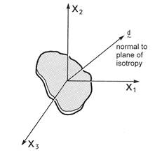
Figure 2.1 Definition of the d vector for local transverse isotropy.

Associated MAC/GMC 4.0 Example Problem(s):

Example 1c-d, Example 2a-d, Example 3a-i, Example 4a-d, Example 4f-h, Example 5e-f, Example 6a-c, Example 7a (see Table 2.2)

Notes:

1) TREF=tref is only required in the special case when the code cannot determine at what temperature the material properties should be taken. This special case occurs when:

· Thermal loading is not specified (*THERM omitted)

– AND –

· Material properties are taken from the internal material database (matid ¹ U)

– OR –

Material properties are user-defined (matid = U) – AND – temperature-dependent

2) In all other cases TREF=tref is optional.

Warning: Specifying TREF=tref will override the temperature dependence and cause the code to employ temperature-independent material properties for the material taken at the temperature tref.

3) D=d₁,d₂,d₃ is only required in the special case when the specified material constitutive model is one that admits arbitrary local transverse isotropy. This occurs when:

cmod=3 – OR – cmod=7 – OR – cmod=9

Additional Information:

MAC/GMC 4.0 Keywords Manual Section 4 (*SOLVER)

MAC/GMC 4.0 Theory Manual Section 4

Table 2.2 MAC/GMC 4.0 constitutive models and internal material property database. Numerical values for the material properties can be obtained from the MAC/GMC output file.

Model	*matid*	Material	Stress Units*	Temperature Dependent?	Example Problem(s)

Bodner-Partom (CMOD=1)	A	Aluminum (2024-T4)	MPa	Yes	2a
	B	Aluminum (2024-0)	MPa	Yes	2a
	C	Aluminum (6061-0) a	MPa	Yes	2a,3c
	D	Aluminum (6061-0) b	MPa	Yes	2a
	E	Aluminum (pure)	MPa	Yes	2a
	F	Titanium (pure)	MPa	No	2a
	G	Copper	MPa	No	2a
	U	User-Defined	–	–	2e,2f,2h

Modified Bodner-Partom (CMOD=2)	A	Ti-21S	MPa	Yes	2b
Modified Bodner-Partom (CMOD=2)	U	User-Defined	–	–	–

Robinson Transversely Isotropic Viscoplastic (CMOD=3)	A	Kanthal	ksi	No (600° C)	–
	B	FeCrAlY	ksi	Yes	–
	C	35% Tungsten/Kanthal Composite	ksi	No (600° C)	–
	U	User-Defined	–	–	–

Isotropic GVIPS (CMOD=4)	A	Ti-21S	ksi	Yes	1c,1d,2b,3a,3b,3d-i,4a-d,4f-h,5e, 5f,6a-c,7a
Isotropic GVIPS (CMOD=4)	U	User-Defined	–	–	2e,3b

Standard Linear Elastic (CMOD=6)	A	Boron Fiber	MPa	No	3c
	B	SiC (SCS-6) Fiber	MPa	Yes	–
	C	Tungsten Fiber	MPa	No	–
	D	Boron Fiber	ksi	No	3a,3b
	E	SiC (SCS-6) Fiber	ksi	Yes	1d,3a,3b,3d-i,4a-d,4f-h, 5e,5f,6-c,7a
	F	Tungsten Fiber	ksi	No	–
	U	User-Defined	–	–	1a,1b,2e,2f,2h,4e,5a-d, 7d,7e

Transversely Isotropic GVIPS (CMOD=7)	A	Ti-6-4	ksi	Yes	–
Transversely Isotropic GVIPS (CMOD=7)	U	User-Defined	–	–	–

Transversely Isotropic Elastic (CMOD=9)	A	T50 Graphite	MPa	No	–
	B	T300 Graphite	MPa	No	–
	C	P100 Graphite	MPa	Yes	–
	D	T50 Graphite	ksi	No	–
	E	T300 Graphite	ksi	No	–
	F	P100 Graphite	ksi	Yes	–
	U	User-Defined	–	–	7b-e

Table 2.2 (continued)


Freed-Walker (CMOD=10)	A	Copper	MPa	Yes	–
	B	NARloy Z	MPa	Yes	–
	U	User-Defined	–	–	–

Robinson Isotropic (CMOD=11)	A	NARloy Z	MPa	Yes	–
Robinson Isotropic (CMOD=11)	U	User-Defined	–	–	–

Anisotropic Elastic (CMOD=15)	U	User-Defined	–	–	7e

Classical Incremental Plasticity (CMOD=21)	A	Copper (bilinear)	MPa	Yes	2c
	B	Ti-24-11 (bilinear)	MPa	Yes	2c
	C	Ti-15-3 (point-wise)	MPa	Yes	2c
	D	Ti-24-11 (point-wise)	MPa	Yes	2c
	E	Copper (bilinear)	ksi	Yes	–
	F	Ti-24-11 (bilinear)	ksi	Yes	–
	G	Ti-15-3 (point-wise)	ksi	Yes	–
	H	Ti-24-11 (point-wise)	ksi	Yes	–
	U	User-Defined	–	–	2e,2f

Multimechanism GVIPS^… (CMOD=22)	A	Ti-21S	ksi	Yes	7a

Shape Memory (CMOD=30)	A	NiTi	MPa	Yes	2d
	B	NiTi	ksi	Yes
	U	User-Defined	–	–

User-Defined (CMOD=99)	U	User-Defined	–	–	2g,2h

* Time units are all seconds, temperature units are all °C, strain is unitless

^… Non-U.S. government users may require an additional software license to use this constitutive model

II. User-defined material properties (matid = U)

A. Material properties read directly from the input file (matdb = 1)

1. Standard constitutive models (cmod¹15, cmod¹99)

Usage:

a) Temperature-independent material properties

*CONSTITUENTS

NMATS=nmats

M=matnum CMOD=cmod TREF=tref MATID=matid MATDB=matdb &

EL=E_A,E_T,n_A,n_T,G_A,a_T,a_A NP=np VI=vi(1),vi(2),…,vi(n) D=d₁,d₂,d₃

K=k_A,k_T

® Repeated nmats times

b) Temperature-dependent material properties

*CONSTITUENTS

NMATS=nmats

M=matnum CMOD=cmod TREF=tref MATID=matid MATDB=matdb

NTP=ntp

TEM=T(1),T(2),…,T(ntp)

EA=E_A(1), E_A(2),…, E_A(ntp)

ET= E_T(1), E_T(2),…, E_T(ntp)

NUA=n_A(1),n_A(2),…,n_A(ntp)

NUT=n_T(1),n_T(2),…,n_T(ntp)

GA=G_A(1),G_A(2),…,G_A(ntp)

ALPA=a_A(1),a_A(2),…,a_A(ntp)

ALPT=a_T(1),a_T(2),…,a_T(ntp)

NP=np

V1=V₁(1), V₁(2),…, V₁(ntp)

V2=V₂(1), V₂(2),…, V₂(ntp)

. ® Repeated n times, where n = number of visco-inelastic properties (see Table 2.3)

Vn=V_n(1), V_n(2),…, V_n(ntp)

KA=k_A(1),k_A(2) ,…,k_A(ntp)

KT=k_T(1),k_T(2) ,…,k_T(ntp)

D=d₁,d₂,d₃

® Repeated nmats times

Name	Definition
nmats	Number of constituent materials specified
matnum	Material number (data following M=matnum is associated with material number matnum) numbered sequentially
cmod	Constitutive model identification number
tref ^1,2	Reference temperature for material (Special Case)
matid [=U]	Material i.d. letter, which indicates location of material parameters = A-H ® Internal material database (see Table 2.2) = U ® User-defined material properties
matdb [=1]	Material database location: = 1 ® Material properties read from input file = 2 ® Material properties determined from user-defined function (usrfun.F90) = 3 ® Material properties read from external material database file
E_A,E_T ³	Axial and transverse elastic (i.e., “Young’s”) modulus
n_A,n_T ³	Axial and transverse Poisson ratios
G_A ³	Axial shear modulus
a_T,a_A ³	Axial and transverse coefficients of thermal expansion (CTEs)
np ⁴	Number of stress-strain points employed to characterize post-yield portion of the stress-strain curve for classical plasticity (Special Case)
vi(1-n) ⁵	Visco-inelastic material properties (Special Case) n = number of visco-inelastic material properties and is cmod dependent ( Table 2.3)
d₁,d₂,d₃ ⁶	Components of vector normal to the plane of transverse isotropy (Special Case) (see Figure 2.1)
k_A,k_T ⁷	Axial and transverse thermal conductivities (Special Case)
ntp	Number of temperatures at which the material properties are specified
T(i)	Temperatures at which the material properties are specified
E_A(i) ³	Axial elastic (i.e., “Young’s”) modulus at input temperature number i
E_T(i) ³	Transverse elastic (i.e., “Young’s”) modulus at input temperature number i
n_A(i) ³	Axial Poisson ratio at input temperature number i
n_T(i) ³	Transverse Poisson ratios at input temperature number i
G_A(i) ³	Axial shear modulus at input temperature number i
a_A(i) ³	Axial coefficient of thermal expansion (CTEs) at input temperature number i
a_T(i) ³	Transverse coefficients of thermal expansion (CTEs) at input temperature number i
V_j(i) ⁵	Visco-inelastic material property number j at input temperature number i (Special Case)
k_A(i) ⁶	Axial thermal conductivity at input temperature number i (Special Case)
k_T(i) ⁶	Transverse thermal conductivity at input temperature number i (Special Case)

Table 2.3 Temperature-independent user-defined inelastic material property specification. See the MAC/GMC 4.0 Theory manual for details on the constitutive models and their parameters.

	n	Inelastic material property specification	Plane of transverse isotropy specification
Bodner-Partom (CMOD=1)	6	VI = D₀, Z₀, Z₁, m, n, q	N/A
Modified Bodner-Partom (CMOD=2)	17	VI = D₀, Z₀, Z₁, Z₂, Z₃, m₁, m₂, n, a₁, a₂, r₁, r₂, Dm₁, Dm₂, Dz₁, Dz₂, Dz₃	N/A
Robinson Transversely Isotropic Viscoplastic (CMOD=3)	10	VI = m, k_T, R, H, n, m, b, h, w,	D=d₁,d₂,d₃
Isotropic GVIPS (CMOD=4)	11	VI = m, k, R_a, B₀, B₁, n, p, q, k₀, B₀’, b	N/A
Standard Linear Elastic (CMOD=6)	N/A	N/A Elastic Only	N/A
Transversely Isotropic GVIPS (CMOD=7)	10	VI = k, n, m, m, b, R, H, G₀, w, h	D=d₁,d₂,d₃
Transversely Isotropic Elastic (CMOD=9)	N/A	N/A Elastic Only	D=d₁,d₂,d₃
Freed-Walker (CMOD=10)	14	VI = A, C, n, Q, T_m, T_t, d, f, h, l, D₀, , ,	N/A
Robinson Isotropic (CMOD=11)	9	VI = A, n, m, b, H, R, K², K₀, G₀	N/A
Anisotropic Elastic (CMOD=15)	N/A	N/A Elastic Only, Special Case – see below	N/A
Classical Plasticity (CMOD=21)	np+1	NP=np VI = s_y, s₁, s₂, … , s_np, e₁, e₂, … , e_np (s_y is the yield stress and s_i,e_i are stress-total strain pairs that characterize the post-yield response)	N/A
Multimechanism GVIPS (CMOD=22)	N/A	N/A Model not currently supported with user-defined properties	N/A
Shape Memory (CMOD=30)	5	VI = f_T, Y, a, a, n	N/A
User-Defined (CMOD=99)	N/A	N/A Special Case – see below	N/A

Examples:

a) Temperature-independent material properties

*CONSTITUENTS

NMATS=2

M=1 CMOD=6 MATID=U MATDB=1 &

EL=388.2E9,7.6E9,0.41,0.45,14.9E9,-0.68E-6,9.74E-6

K=500.,10.

M=2 CMOD=6 MATID=U MATDB=1 &

EL=3.45E9,3.45E9,0.35,0.35,1.278E9,45.E-6,45.E-6

K=0.19,0.19

*CONSTITUENTS

NMATS=5

M=1 CMOD=1 MATID=U MATDB=1 &

EL=9.53E3,9.53E3,0.33,0.33,3.58E3,21.06E-6,21.06E-6 &

VI=1.E4,49.,63.,300.,4.,1.

M=2 CMOD=9 MATID=U MATDB=1 &

EL=253.5E9,6.05E9,0.39,0.47,4.167E9,-0.4724E-6,26.63E-6 D=0.5,1.,0.

M=3 CMOD=4 MATID=U MATDB=1 &

EL=14009.,14009.,0.365,0.365,5131.5,5.862E-6,5.862E-6 &

VI=0.000999275,44.960,1.679E-07,2.494561E-05,0.05, &

3.3,1.8,1.35,0.85,3.0183E-7,0.001

M=4 CMOD=10 MATID=U MATDB=1 &

EL=0.1305E+06,0.1305E+06,0.36,0.36,0.4798E+05,0.165E-04,0.165E-04 &

VI=0.2000E+08,0.1300E+02,0.4500E+01,0.2000E+06,1082.85, &

404.85,0.3500E-01,0.5000E+00,0.4000E+02,0.6500E+01, &

0.1300E+00,0.1000E-01,0.1000E-06,0.7000E+00

M=5 CMOD=21 MATID=U MATDB=1 &

EL=10000.,10000.,0.326,0.326,3770.,12.00E-6,12.00E-6 &

NP=1 VI=5.08,13.1,0.15

b) Temperature-dependent material properties

*CONSTITUENTS

NMATS=2

M=1 CMOD=21 MATID=U MATDB=1

NTP=3

TEM=21.,400.,800.

EA=10000.,9000.,7300.

ET=10000.,9000.,7300.

NUA=0.326,0.351,0.345

NUT=0.326,0.351,0.345

GA=3771.,3331.,2714.

ALPA=12.00E-6,13.50E-6,22.72E-6

ALPT=12.00E-6,13.50E-6,22.72E-6

NP=3

V1=4.20,3.81,3.05

V2=6.13,4.77,3.69

V3=6.60,5.10,3.90

V4=13.1,9.70,5.10

V5=0.004,0.004,0.004

V6=0.01,0.01,0.01

V7=0.15,0.15,0.15

M=2 CMOD=1 MATID=U MATDB=1

NTP=2

TEM=18.,700.

EA=9.53E3,4.12E3

ET=9.53E3,4.12E3

NUA=0.41,0.41

NUT=0.41,0.41

GA=3.58E3,1.46E3

ALPA=21.06E-6,28.92E-6

ALPT=21.06E-6,28.92E-6

V1=1.E4,1.E4

V2=49.,49.

V3=63.,63.

V4=300.,300.

V5=4.,2.5

V6=1.,1.

Associated MAC/GMC 4.0 Example Problem(s):

a) Temperature-independent material properties

Example 1a, Example 1b, Example 2e, Example 3b, Example 7e

b) Temperature-dependent material properties

Example 2e, Example 4e, Example 5a, Example 5b, Example 5c, Example 5d

Additional Information:

MAC/GMC 4.0 Keywords Manual Section 4 (*SOLVER)

MAC/GMC 4.0 Theory Manual Section 4

2. Special cases

a) Internal anisotropic constitutive model (cmod=15)

Usage:

i) Temperature-independent material properties

*CONSTITUENTS

NMATS=nmats

M=matnum CMOD=cmod TREF=tref MATID=matid MATDB=matdb &

EL=C₁₁,C₁₂,C₁₃,C₁₄,C₁₅,C₁₆,C₂₂,C₂₃,C₂₄,C₂₅,C₂₆,C₃₃,C₃₄,C₃₅,C₃₆,C₄₄,C₄₅,C₄₆,C₅₅,C₅₆,C₆₆, &

a₁₁, a₂₂, a₃₃,a₂₃,a₁₃,a₁₂

® Repeated nmats times

ii) Temperature-independent material properties

*CONSTITUENTS

NMATS=nmats

M=matnum CMOD=cmod TREF=tref MATID=matid MATDB=matdb

NTP=ntp

TEM=T(1),T(2),…,T(ntp)

C11=C₁₁(1),C₁₁(2),…,C₁₁(ntp)

C12=C₁₂(1),C₁₂(2),…,C₁₂(ntp)

C13=C₁₃(1),C₁₃(2),…,C₁₂(ntp)

C14=C₁₄(1),C₁₄(2),…,C₁₄(ntp)

C15=C₁₅(1),C₁₅(2),…,C₁₅(ntp)

C16=C₁₆(1),C₁₆(2),…,C₁₆(ntp)

C22=C₂₂(1),C₂₂(2),…,C₂₂(ntp)

C23=C₂₃(1),C₂₃(2),…,C₂₃(ntp)

C24=C₂₄(1),C₂₄(2),…,C₂₄(ntp)

C25=C₂₅(1),C₂₅(2),…,C₂₅(ntp)

C26=C₂₆(1),C₂₆(2),…,C₂₆(ntp)

C33=C₃₃(1),C₃₃(2),…,C₃₃(ntp)

C34=C₃₄(1),C₃₄(2),…,C₃₄(ntp)

C35=C₃₅(1),C₃₅(2),…,C₃₅(ntp)

C36=C₃₆(1),C₃₆(2),…,C₃₆(ntp)

C44=C₄₄(1),C₄₄(2),…,C₄₄(ntp)

C45=C₄₅(1),C₄₅(2),…,C₄₅(ntp)

C46=C₄₆(1),C₄₆(2),…,C₄₆(ntp)

C55=C₅₅(1),C₅₅(2),…,C₅₅(ntp)

C56=C₅₆(1),C₅₆(2),…,C₅₆(ntp)

C66=C₆₆(1),C₆₆(2),…,C₆₆(ntp)

ALF1=a₁₁(1),a₁₁(2),…,a₁₁(ntp)

ALF2=a₂₂(1),a₂₂(2),…,a₂₂(ntp)

ALF3=a₃₃(1),a₃₃(2),…,a₃₃(ntp)

ALF4=a₂₃(1),a₂₃(2),…,a₂₃(ntp)

ALF5=a₁₃(1),a₁₃(2),…,a₁₃(ntp)

ALF6=a₁₂(1),a₁₂(2),…,a₁₂(ntp)

® Repeated nmats times

Name	Definition
nmats	Number of constituent materials specified
matnum	Material number (data following M=matnum is associated with material number matnum) numbered sequentially
cmod [=15]	Constitutive model identification number
tref ^1,2	Reference temperature for material (Special Case)
Name	Definition
matid [=U]	Material i.d. letter, which indicates location of material parameters = A-H ® Internal material database (see Table 2.2) = U ® User-defined material properties
matdb [=1]	Material database location: = 1 ® Material properties read from input file = 2 ® Material properties determined from user-defined function (usrfun.F90) = 3 ® Material properties read from external material database file
C_ij	Stiffness matrix coefficients
a_ij ³	CTE vector components (anisotropic materials can have 6 CTE components)
ntp	Number of temperatures at which the material properties are specified
T(i)	Temperatures at which the material properties are specified
C_jk(i)	Stiffness matrix component jk at input temperature number i
a_jk(i) ³	CTE component jk at input temperature number i

Examples:

i) Temperature-independent material properties

*CONSTITUENTS

NMATS=1

M=1 CMOD=15 MATID=U MATDB=1 &

EL=6.677E9, 3.274E9, 4.843E9, 0., -0.1887E9, 0., &

6.662E9, 3.384E9, 0., 0.006711E9, 0., &

55.80E9, 0., -6.969E9, 0., &

2.625E9, 0., -0.1830E9, &

2.269E9, 0., &

1.613E9 &

43.74E-6, 39.04E-6, 4.043E-6, 0., 12.19E-6, 0.

ii) Temperature-dependent material properties

*CONSTITUENTS

NMATS=1

M=1 CMOD=15 MATID=U MATDB=1

NTP=2

TEM=23.,250.

C11=6.677E9,5.973E9

C12=3.274E9,2.931E9

C13=4.843E9,4.517E9

C14=0.,0.

C15=0.1887E9,0.1932E9

C16=0.,0.

C22=6.662E9,5.867E9

C23=3.384E9,3.023E9

C24=0.,0.

C25=-0.006711E9,0.008475E9

C26=0.,0.

C33=55.80E9,48.22E9

C34=0.,0.

C35=6.969E9,7.105E9

C36=0.,0.

C44=2.625E9,2.124E9

C45=0.,0.

C46=0.1830E9,0.1363E9

C55=2.269E9,2.123E9

C56=0.,0.

C66=1.613E9,1.444E9

ALF1=43.74E-6,46.75E-6

ALF2=39.04E-6,43.81E-6

ALF3=4.043E-6,5.241E-6

ALF4=0.,0.

ALF5=-12.19E-6,-16.45E-6

ALF6=0.,0.

Associated MAC/GMC 4.0 Example Problem(s):

Example 7e

Additional Information:

MAC/GMC 4.0 Keywords Manual Section 4 (*SOLVER)

b) User-defined constitutive model (cmod=99)

Usage:

i) Temperature-independent material properties

*CONSTITUENTS

NMATS=nmats

M=matnum CMOD=cmod TREF=tref MATID=matid MATDB=matdb NPE=npe NPV=npv &

EL=E(1),E(2),…,E(npe) ALP=α_A,α_T VI=V(1),V(2),…,V(npv)

K=k_A,k_T

® Repeated nmats times

ii) Temperature-dependent material properties

*CONSTITUENTS

NMATS=nmats

M=matnum CMOD=cmod TREF=tref MATID=matid MATDB=matdb

NPE=npe NPV=npv

NTP=ntp

TEM=T(1),T(2),…,T(ntp)

E1=E₁(1), E₁(2),…, E₁(ntp)

E2= E₂(1), E₂(2),…, E₂(ntp)

. ® Repeated npe times

Envp=E_nvp(1), E_nvp(2),…, E_nvp(ntp)

ALPA=a_A(1),a_A(2),…,a_A(ntp)

ALPT=a_T(1),a_T(2),…,a_T(ntp)

V1=V₁(1), V₁(2),…, V₁(ntp)

V2=V₂(1), V₂(2),…, V₂(ntp)

. ® Repeated npv times

Vnvp=V_nvp(1), V_nvp(2),…, V_nvp(ntp)

KA=k_A(1),k_A(2) ,…,k_A(ntp)

KT=k_T(1),k_T(2) ,…,k_T(ntp)

® Repeated nmats times

Name	Definition
nmats	Number of constituent materials specified
matnum	Material number (data following M=matnum is associated with material number matnum) numbered sequentially
cmod [=99] ^9,10	Constitutive model identification number
tref ^1,2	Reference temperature for material (Special Case)
matid [=U]	Material i.d. letter, which indicates location of material parameters = A-H ® Internal material database (see Table 2.2) = U ® User-defined material properties
matdb [=1]	Material database location: = 1 ® Material properties read from input file = 2 ® Material properties determined from user-defined function (usrfun.F90) = 3 ® Material properties read from external material database file
npe	Number of elastic constants employed in user-defined constitutive model
npv ⁴	Number of visco-inelastic constants employed in user-defined constitutive model
E(1-npe)	Elastic constants
α_A,α_T	Axial and transverse coefficients of thermal expansion (CTEs)
V(1-npv) ⁴	Visco-inelastic constants
k_A,k_T ⁷	Axial and transverse thermal conductivities (Special Case)
ntp	Number of temperatures at which the material properties are specified
T(i)	Temperatures at which the material properties are specified
E_j(i)	Elastic material property number j at input temperature number i
a_A(i)	Axial coefficient of thermal expansion (CTEs) at input temperature number i
a_T(i)	Transverse coefficients of thermal expansion (CTEs) at input temperature number i
V_j(i) ¹¹	Visco-inelastic material property number j at input temperature number i
k_A(i) ⁷	Axial thermal conductivity at input temperature number i (Special Case)
k_T(i) ⁷	Transverse thermal conductivity at input temperature number i (Special Case)

Examples:

i) Temperature-independent material properties

*CONSTITUENTS

NMATS=2

M=1 CMOD=99 MATID=U MATDB=1 NPE=2 NPV=2 &

EL=55.2E9,0.30 ALP=22.5E-6,22.5E-6 VI=1.5E-28,3.0

K=273.,273.

M=2 CMOD=99 MATID=U MATDB=1 NPE=2 NPV=6 &

EL=55.2E9,0.30 ALP=22.5E-6,22.5E-6 &

VI=1000.,103.42E6,103.42E6,1700.,10.,1.0

K=273.,273.

ii) Temperature-dependent material properties

*CONSTITUENTS

NMATS=1

M=1 CMOD=99 MATID=U MATDB=1

NPE=2 NPV=2

NTP=3

TEM=21.,350.,650.

E1=55.2E9,52.7E9,47.1E9

E2=0.30,0.30,0.30

ALPA=22.5E-6,23.4E-6,27.0E-6

ALPT=22.5E-6,23.4E-6,27.0E-6

V1=1.5E-28,1.5E-28,1.5E-28

V2=3.0,3.017,3.052

Associated MAC/GMC 4.0 Example Problem(s):

Example 2g

Additional Information:

MAC/GMC 4.0 Keywords Manual Appendix

Notes:

1) TREF=tref is only required in the special case when the code cannot determine at what temperature the material properties should be taken. This special case occurs when:

· Thermal loading is not specified (*THERM omitted)

– AND –

· Material properties are taken from the internal material database (matid ¹ U)

– OR –

Material properties are user-defined (matid = U) – AND – temperature-dependent

2) In all other cases TREF=tref is optional.

Warning: Specifying TREF=tref will override the temperature dependence and cause the code to employ temperature-independent material properties for the material taken at the temperature tref.

3) To obtain isotropic material behavior, set, E_A = E_T, n_A = n_T, G_A = E_A / 2(1+n_A), and a_A = a_T.

4) NP=np is only required in the special case that the material constitutive model is classical incremental plasticity (cmod=21). A maximum value of NP=9 may be specified.

5) The lines associated with the visco-inelastic material properties (VI= vi(1),…, V_j= V_j(i),…) are only required in the special case when the constitutive model (cmod) chosen is an inelastic model. This occurs when:

cmod¹6 – AND – cmod¹9 – AND – cmod¹15

6) D=d₁,d₂,d₃ is only required in the special case when the specified material constitutive model is on e that admits local transverse isotropy. This occurs when:

cmod=3 – OR – cmod=7 – AND – cmod=9

7) The thermal conductivity specifiers (K=k_A,k_T, KA=k_A,…, KT=k_T,…) are only required in the special case when the code is calculating effective thermal conductivities of the RUC. This occurs when the *CONDUCTIVITY keyword is specified. The thermal conductivity specification is only valid for materials that are isotropic or transversely isotropic with an x₂-x₃ plane of isotropy (in the global RUC coordinates).

8) Shear CTEs are engineering quantities. That is, for example, .

9) When a user-defined constitutive model is selected (CMOD=99), MAC/GMC 4.0 will use the code in the file usrmat.F90 to determine the inelastic strain increments for any subcells contain that particular material. The MAC/GMC 4.0 executable that is distributed has been linked with the demonstration usrmat subroutine, the source code of which is also distributed with MAC/GMC 4.0 (see Appendix). In order for users to employ their own usrmat subroutine, it is necessary to place the appropriate code in the usrmat.F90 file and to compile the subroutine and link with the MAC/GMC 4.0 library file (mac4.lib), which is also distributed with MAC/GMC 4.0. This procedure results in a new MAC/GMC 4.0 executable file that is now linked to the user’s own usrmat subroutine rather than the demonstration version of usrmat distributed with the code. It is the user’s responsibility to ensure that the coding, compilation, and linking of the user’s own usrmat subroutine is done correctly and that the desired user-defined constitutive model is actually being employed when the code is executed. A printout of the demonstration usrmat subroutine that is distributed with MAC/GMC 4.0 is given in the Appendix of this manual. Note that when the code executes the demonstration version of the usrmat subroutine, a message is printed to the screen.

10) When a user-defined constitutive model is selected (CMOD=99), MAC/GMC 4.0 will use the code in the file usrformde.F90 to calculate the material elastic stiffness matrix from the user-defined elastic properties. This is necessary because the user is free to employ any elastic constants desired (e.g., Lamé constants, compliance components). Thus the code does not (in general) know how to form the stiffness matrix from the user’s elastic constants. As with the usrmat file, the MAC/GMC 4.0 executable that is distributed has been linked with a demonstration usrformde subroutine, the source code of which is also distributed with MAC/GMC 4.0 (see Appendix). It is the user’s responsibility to ensure that the coding, compilation, and linking of the user’s own usrformde subroutine is done correctly and that the stiffness matrix of the user’s material is being calculated correctly when the code is executed. A printout of the demonstration usrformde subroutine that is distributed with MAC/GMC 4.0 is given in the Appendix of this manual. Note that when the code executes the demonstration version of the usrformde subroutine, a message is printed to the screen.

11) For a user-defined elastic constitutive model, set npv = 0 and omit the V1 – Vnvp lines.

B. Material properties determined from a user-defined function (matdb = 2)

Usage:

*CONSTITUENTS

NMATS=nmats

M=matnum CMOD=cmod TREF=tref MATID=matid MATDB=matdb

® Repeated nmats times

Name	Definition
nmats	Number of constituent materials specified
matnum	Material number (data following M=matnum is associated with material number matnum) numbered sequentially
cmod	Constitutive model identification number
tref ^1,2	Reference temperature for material (Special Case)
matid [=U]	Material i.d. letter, which indicates location of material parameters = A-H ® Internal material database (see Table 2.2) = U ® User-defined material properties
matdb [=2] ^3,4	Material database location: = 1 ® Material properties read from input file = 2 ® Material properties determined from user-defined function (usrfun.F90) = 3 ® Material properties read from external material database file

Example:

*CONSTITUENTS

NMATS=5

M=1 CMOD=6 MATID=U MATDB=2

M=2 CMOD=21 MATID=U MATDB=2

M=3 CMOD=1 TREF=650. MATID=U MATDB=2

M=4 CMOD=1 TREF=650. MATID=U MATDB=2

M=5 CMOD=99 MATID=U MATDB=2

Associated MAC/GMC 4.0 Example Problem(s):

Example 2f

Notes:

1) TREF=tref is only required in the special case when the code cannot determine at what temperature the material properties should be taken. This special case occurs when:

· Thermal loading is not specified (*THERM omitted)

– AND –

· Material properties are taken from the internal material database (matid ¹ U)

– OR –

Material properties are user-defined (matid = U) – AND – temperature-dependent

2) In all other cases TREF=tref is optional.

Warning: Specifying TREF=tref will override the temperature dependence and cause the code to employ temperature-independent material properties for the material taken at the temperature tref.

3) When a user-defined function is selected to determine a material’s properties (MATDB=2), MAC/GMC 4.0 will use the code in the file usrfun.F90 to determine the material properties at every increment of the simulated applied loading. The MAC/GMC 4.0 executable that is distributed has been linked with the demonstration usrfun subroutine, the source code of which is also distributed with MAC/GMC 4.0 (see Appendix). In order for users to employ their own usrfun subroutine, it is necessary to place the appropriate code in the usrfun.F90 file and to compile the subroutine and link with the MAC/GMC 4.0 library file (mac4.lib), which is also distributed with MAC/GMC 4.0. This procedure results in a new MAC/GMC 4.0 executable file that is now linked to the user’s own usrfun subroutine rather than the demonstration version of usrfun distributed with the code. It is the user’s responsibility to ensure that the coding, compilation, and linking of the user’s own usrfun subroutine is done correctly and that the desired user-defined function is actually being employed when the code is executed. A printout of the demonstration usrfun subroutine that is distributed with MAC/GMC 4.0 is given in the Appendix of this manual. Note that when the code executes the demonstration version of the usrfun subroutine, a message is printed to the screen. The usrfun subroutine can be used to allow the elastic and inelastic material properties to be a function of temperature or another variable. It works in concert with the MAC/GMC internal constitutive models as well as the user-defined constitutive model subroutine (usrmat).

4) In MAC/GMC 4.0, the material properties are associated with constituent materials as opposed to subcells. That is, several subcells may contain material number 1, and thus all of those subcells must have the same material properties. This is relevant when employing the usrfun.F90 subroutine to make material properties a function of field variables (as is done in Example Problem 2f). If, for instance, the properties of material number 1 are determined from a function of strain and material number 1 is placed in two subcells, the subcells will in general experience different strain states. It is thus impossible for material number 1 to have the correct material properties to correspond to the two different states of strain in each subcell. For this reason, when material properties are determined from a function of field variables (other than temperature, which does not vary within the repeating unit cell), each subcell should be given its own material.

Additional Information:

MAC/GMC 4.0 Keywords Manual Appendix

C. Material properties read from external material database file (matdb = 3)

Usage:

*CONSTITUENTS

NMATS=nmats

M=matnum CMOD=cmod TREF=tref MATID=matid MATDB=matdb EXTMAT=matname

® Repeated nmats times

Name	Definition
nmats	Number of constituent materials specified
matnum	Material number (data following M=matnum is associated with material number matnum) numbered sequentially
cmod	Constitutive model identification number
tref ^1,2	Reference temperature for material (Special Case)
matid [=U]	Material i.d. letter, which indicates location of material parameters = A-H ® Internal material database (see Table 2.2) = U ® User-defined material properties
matid [=U]	Material i.d. letter from internal material database
matdb [=3] ³	Material database location: = 1 ® Material properties read from input file = 2 ® Material properties determined from user-defined function (usrfun.F90) = 3 ® Material properties read from external material database file
matname ⁴	Name of material in external material database file

Examples:

*CONSTITUENTS

NMATS=3

M=1 CMOD=1 MATID=U MATDB=3 EXTMAT=copper

M=2 CMOD=99 MATID=U MATDB=3 EXTMAT=Al(6061-0)

M=3 CMOD=6 MATID=U MATDB=3 EXTMAT=SCS-6

Example portion of the external material database file:

# ------- Bodner-Partom Model Material

MAT=copper

CMOD=1

EL=120.E9,120.E9,0.33,0.33,45.11E9,14.7E-6,14.7E-6 &

VI=1.E4,63.E6,250.E6,8.19,7.5,0.55

K=1.,2.

Associated MAC/GMC 4.0 Example Problem(s):

Example 2h

Notes:

1) TREF=tref is only required in the special case when the code cannot determine at what temperature the material properties should be taken. This special case occurs when:

· Thermal loading is not specified (*THERM omitted)

– AND –

· Material properties are taken from the internal material database (matid ¹ U)

– OR –

Material properties are user-defined (matid = U) – AND – temperature-dependent

2) In all other cases TREF=tref is optional.

Warning: Specifying TREF=tref will override the temperature dependence and cause the code to employ temperature-independent material properties for the material taken at the temperature tref.

3) In order to use the external material database feature of MAC/GMC 4.0, the *MDBPATH keyword must be specified (see Section 1 of this manual). It is there that the name of the external material database file is specified.

4) The format of the material property specification in the external material database file is very similar to that employed in the MAC/GMC 4.0 input file for user-defined material properties. A printout of the sample external material database file distributed with MAC/GMC 4.0 is given in the appendix of this manual. The same special characters (“#” for a comment, “&” for a continuation) that can be used in the input file can be used in the external material database file, and the first line of the file is interpreted as a title. Each material in the file is specified by a name using the line:

MAT=matname

where matname is the name of the material. The matname specified in the input file should correspond to one (and only one) of the material names in the external material database file. The next line for each material re-specifies the material constitutive model:

CMOD=cmod

The code uses this as a consistency check as it must match the value of cmod specified for the material in the input file. The remainder of the material property input data in the external material database file follows the format of the user-defined material properties that read directly from the input file (see outline section II. A. above)

Additional Information:

MAC/GMC 4.0 Keywords Manual Section 2 (*MDBPATH)

MAC/GMC 4.0 Keywords Manual Appendix

III. Electromagnetic (smart) material properties

Usage:

A) Temperature-independent electromagnetic material properties

*CONSTITUENTS

NMATS=nmats

M=matnum CMOD=cmod TREF=tref MATID=matid MATDB=matdb EM=em &

EL=E_A,E_T,n_A,n_T,G_A,a_T,a_A D=d₁,d₂,d₃

ES=e₁₁,e₁₂,e₂₆

QS=q₁₁,q₁₂,q₂₆

KS=k₁₁, k₂₂

AS=a₁₁,a₂₂

MS=m₁₁, m₂₂

PELS=z₁, z₂

PMGS=y₁, y₁

® Repeated nmats times

B) Temperature-dependent electromagnetic material properties

*CONSTITUENTS

NMATS=nmats

M=matnum CMOD=cmod TREF=tref MATID=matid MATDB=matdb EM=em

NTP=ntp

TEM=T(1),T(2),…,T(ntp)

EA=E_A(1), E_A(2),…, E_A(ntp)

ET= E_T(1), E_T(2),…, E_T(ntp)

NUA=n_A(1),n_A(2),…,n_A(ntp)

NUT=n_T(1),n_T(2),…,n_T(ntp)

GA=G_A(1),G_A(2),…,G_A(ntp)

ALPA=a_A(1),a_A(2),…,a_A(ntp)

ALPT=a_T(1),a_T(2),…,a_T(ntp)

D=d₁,d₂,d₃

ES11=e₁₁(1),e₁₁(2),…,e₁₁(ntp)

ES12=e₁₂(1),e₁₂(2),…,e₁₂(ntp)

ES26=e₂₆(1),e₂₆(2),…,e₂₆(ntp)

QS11=q₁₁(1),q₁₁(2),…,q₁₁(ntp)

QS12=q₁₂(1),q₁₂(2),…,q₁₂(ntp)

QS26=q₂₆(1),q₂₆(2),…,q₂₆(ntp)

KS11=k₁₁(1),k₁₁(2),…,k₁₁(ntp)

KS22=k₂₂(1),k₂₂(2),…,k₂₂(ntp)

AS11=a₁₁(1),a₁₁(2),…,a₁₁(ntp)

AS22=a₂₂(1),a₂₂(2),…,a₂₂(ntp)

MS11=m₁₁(1),m₁₁(2),…,m₁₁(ntp)

MS22=a₂₂(1),m₂₂(2),…,m₂₂(ntp)

PELS1=z₁(1),z₁(2),…,z₁(ntp)

PELS2=z₂(1),z₂(2),…,z₂(ntp)

PMGS1=y₁(1),y₁(2),…,y₁(ntp)

PMGS2=y₂(1),y₂(2),…,y₂(ntp)

® Repeated nmats times

Name	Definition
nmats	Number of constituent materials specified
matnum	Material number (data following M=matnum is associated with material number matnum) numbered sequentially
cmod [=9] ¹	Constitutive model identification number
tref ^2,3	Reference temperature for material (Special Case)
matid [=U]	Material i.d. letter, which indicates location of material parameters = A-H ® Internal material database (see Table 2.2) = U ® User-defined material properties
matdb [=1] ¹	Material database location: = 1 ® Material properties read from input file = 2 ® Material properties determined from user-defined function (usrfun.F90) = 3 ® Material properties read from external material database file
em [=1] ⁴	Electromagnetic specifier for material: = 0 ® Material is not electromagnetic = 1 ® Material is electromagnetic
E_A,E_T	Axial and transverse elastic (i.e., “Young’s”) modulus
n_A,n_T	Axial and transverse Poisson ratios
G_A	Axial shear modulus
a_T,a_A	Axial and transverse coefficients of thermal expansion (CTEs)
d₁,d₂,d₃ ⁵	Components of vector normal to the plane of transverse isotropy (see Figure 2.1)
e_kj	Material piezoelectric component kj
q_kj	Material piezomagnetic component kj
k_ij	Material dielectric component ij
a_ij	Material magnetoelectric component ij
m_ij	Material magnetic permeability component ij
z_k	Material pyroelectric constant component k
y_k	Material pyromagnetic constant component k
E_A(p)	Axial elastic (i.e., “Young’s”) modulus at input temperature number p
E_T(p)	Transverse elastic (i.e., “Young’s”) modulus at input temperature number p
n_A(p)	Axial Poisson ratio at input temperature number p
n_T(p)	Transverse Poisson ratios at input temperature number p
G_A(p)	Axial shear modulus at input temperature number p
a_A(p)	Axial coefficient of thermal expansion (CTEs) at input temperature number p
a_T(p)	Transverse coefficients of thermal expansion (CTEs) at input temperature number p
d₁,d₂,d₃ ⁵	Components of vector normal to the plane of transverse isotropy (see Figure 2.1)
e_kj(p)	Material piezoelectric component kj at input temperature number p
q_kj(p)	Material piezomagnetic component kj at input temperature number p
Name	Definition
k_ij(p)	Material dielectric component ij at input temperature number p
a_ij(p)	Material magnetoelectric component ij at input temperature number p
m_ij(p)	Material magnetic permeability component ij at input temperature number p
z_k(p)	Material pyroelectric constant component k at input temperature number p
y_k(p)	Material pyromagnetic constant component k at input temperature number p

Examples:

A) Temperature-independent electromagnetic material properties

*CONSTITUENTS

NMATS=1

M=1 CMOD=9 MATID=U MATDB=1 EM=1 &

EL=143.57E9,154.57E9,0.37,0.368,45.3E9,0.00E-6,0.00E-6 &

D=0.,0.,1.

ES=0.0,0.0,0.0

QS=699.7,580.3,550.

KS=0.93E-10,0.08E-9

AS=0.0,0.0

MS=157.E-6,-590.E-6

PELS=0.0,0.0

PMGS=0.0,0.0

B) Temperature-dependent electromagnetic material properties

*CONSTITUENTS

NMATS=2

M=1 CMOD=9 MATID=U MATDB=1 EM=1

NTP=2

TEM=24.,600.

EA=111.93E9,101.43E9

ET=116.33E9,107.10E9

NUA=0.321,0.321

NUT=0.307,0.307

GA=43.0E9,41.5E9

ALPA=1.99E-6,2.55E-6

ALPT=8.53E-6,10.80E-6

D=0.,0.,1.

ES11=18.6,18.6

ES12=-4.4,-4.4

ES26=11.6,11.6

QS11=0.0,0.0

QS12=0.0,0.0

QS26=0.0,0.0

KS11=12.6E-9,12.6E-9

KS22=11.2E-9,11.2E-9

AS11=0.0,0.0

AS22=0.0,0.0

MS11=10.0E-6,10.0E-6

MS22=5.0E-6,5.0E-6

PELS1=0.13E5,0.13E5

PELS2=0.13E5,0.13E5

PMGS1=0.0,0.0

PMGS2=0.0,0.0

Associated MAC/GMC 4.0 Example Problem(s):

Example 7b, Example 7c

Notes:

1) In order to perform coupled thermo-electro-magneto-elasto-plastic analysis of smart composites and laminates, the *ELECTROMAG keyword must be specified (see Section 1 of this example manual). Further, the coupled analysis requires the constituent materials to have certain additional electromagnetic properties. Currently, specification of these properties is limited in MAC/GMC 4.0 to the case in which:

a) The material constitutive model is the transversely isotropic elastic model (cmod=9)

– AND –

b) The material properties are user-defined (matid=U)

– AND –

c) The material properties are read from the input file (matdb=1)

Thus, the specification of constituent electromagnetic properties actually falls within section II. A. of this outline rather than in its own section III. The present format was chosen for simplicity and so as to make the electromagnetic property section more evident to the reader.

2) TREF=tref is only required in the special case when the code cannot determine at what temperature the material properties should be taken. This special case occurs when:

· Thermal loading is not specified (*THERM omitted)

– AND –

· Material properties are taken from the internal material database (matid ¹ U)

– OR –

Material properties are user-defined (matid = U) – AND – temperature-dependent

3) In all other cases TREF=tref is optional.

Warning: Specifying TREF=tref will override the temperature dependence and cause the code to employ temperature-independent material properties for the material taken at the temperature tref.

4) The electromagnetic specifier (EM=em) is required to indicate if a particular material is electromagnetically active (i.e., if it has electromagnetic properties). This allows electromagnetically active and inactive constitutents to both be present in a composite or laminate.

5) D=d₁,d₂,d₃ is required when the material is electromagnetically active (EM=1) because, in such a case, the transversely isotropic elastic model must be employed (cmod=9).

Additional Information:

MAC/GMC 4.0 Keywords Manual Section 2 (*ELECTROMAG)

MAC/GMC 4.0 Keywords Manual Section 4 (*LAMINATE)

MAC/GMC 4.0 Keywords Manual Section 4 (*MECH)

MAC/GMC 4.0 Theory Manual Section 2.2.2

Section 3 : Analysis Type and Architecture Keywords

This section deals with the keywords used to select the overall analysis type and the particular micromechanics model(s) that will be used by MAC/GMC 4.0 to analyze the particular problem. The two MAC/GMC 4.0 input file keywords covered in this section are:

*RUC ® Invokes repeating unit cell (RUC) analysis, that is, models the behavior of a composite material (continuum)

*LAMINATE ® Invokes laminate analysis, therefore models the behavior of a composite laminate (finite in one direction) with access to individual ply, RUC, and subcell data

RUC analysis allows simulations to be performed on a heterogeneous (composite) material that is represented by a repeating unit cell. There are three separate micromechanics models within MAC/GMC 4.0 that can be employed in RUC analyses: 1) Doubly periodic generalized method of cells (GMC), 2) Triply periodic GMC, and 3) Doubly periodic high-fidelity GMC (HFGMC). The doubly periodic GMC RUC is shown in Figure 3.1, while the triply periodic GMC RUC is shown in Figure 3.2. The RUC for doubly periodic HFGMC is identical to that of doubly-periodic GMC with the current restriction that the number of subcells in each direction must be even. By assigning the different constituent materials (specified under *CONSTITUENTS) to the subcells within the RUC, the RUC can be constructed to represent a composite material with the desired architecture. As the name indicates, the RUC repeats infinitely in either two (doubly periodic) or three (triply periodic) Cartesian coordinate directions. The doubly periodic RUC is infinitely long in the third (out-of-plane) x₁-direction (see Figure 3.1), so both RUCs represent an infinite heterogeneous (composite) medium with a periodic microstructure. Thus, GMC and HFGMC may be thought of as models for a material point that may be part of a larger overall structure. These micromechanics models not only calculate the effective properties of the composite material located at a particular material point, but also allow the simulation of applied loading (in the form of global stresses, global strains, a uniform temperature change, and electromagnetic loads) on the composite material (see Section 4 of this manual).

Laminate analysis, on the other hand, simulates the behavior of a structure, namely a laminated plate. MAC/GMC 4.0 employs classical lamination theory (Jones, 1975; Herakovich, 1998) to model the composite laminate as infinite in the in-plane x- and y-directions and finite in the through-thickness z-direction (see Figure 3.3). Simulated loading for the laminate takes the form of in-plane stress and moment resultants and midplane strains and curvatures (see Section 4 of this manual). As Figure 3.3 indicates, each ply of the laminate may be a composite material, which is then represented by a doubly or triply periodic GMC RUC. The GMC micromechanics models are thus embedded within the laminate theory analysis to represent the composite material points within the laminate plies. In the presence of laminate bending and inelastic material behavior, the stress and strain fields in the laminate will vary nonlinearly in the through-thickness (z-) direction. In such a case, MAC/GMC 4.0 tracks the fields in the laminate at two Gauss quadrature (integration) points in each layer (see Figure 3.3). During incremental application of the applied laminate-level simulated loading, the appropriate GMC micromechanics model is called at each of the two integration points in each layer to determine the local inelastic behavior of the composite material. The local inelastic behavior represented by the quadrature points can then be employed to determine the laminate level inelastic effects, which accounted for as inelastic force and moment resultants (see the MAC/GMC 4.0 Theory Manual Section 3).

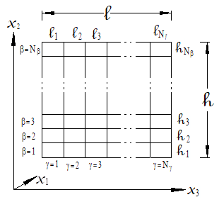
Figure 3.1 Doubly periodic GMC and HFGMC repeating unit cell (RUC). The RUC is composed of subcells, each of which contains a constituent material. The subcells are identified by the indices bg. Note that for HFGMC, N_β and N_γ must be even.

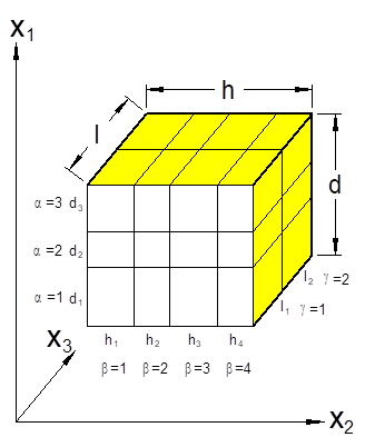
Figure 3.2 Triply periodic GMC repeating unit cell (RUC). The RUC is composed of subcells, each of which contains a constituent material. The subcells are identified by the indices abg.

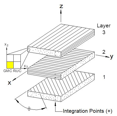
Figure 3.3 Geometry employed in MAC/GMC 4.0 for laminate theory analysis. Each ply is represented by a doubly or triply periodic GMC repeating unit cell (RUC), which operate at the Gauss quadrature points.

*RUC: Repeating unit cell analysis and architecture

P Either *RUC or *LAMINATE is required in all input files P

Purpose:

Invoke repeating unit cell analysis (as opposed to laminate analysis) for the problem, which requires the selection of the micromechanics model used to analyze the RUC and specification of the RUC architecture (i.e., arrangement of the composite constituents).

The RUC section is broken into two sub-sections:

I. Internal RUC Architecture Library (archid≠99)

II. User-Defined RUC Architecture (archid=99)

I. Internal RUC Architecture Library (archid≠99)

Usage:

*RUC

MOD=modid ARCHID=archid ® specifics: see Table 3.1 and Table 3.2 ¬

Table 3.1 Specific input data for the internal doubly periodic RUC architecture library.

Architecture		Specific Data Input Format
0	Monolithic Material	*RUC MOD=2 ARCHID=0 M=mm
1	Square Fiber, Square Pack	*RUC MOD=2 ARCHID=1 VF=vf RAD=rad RITFR=ritfr F=mf M=mm I=mi
2	Square Fiber, Hexagonal Pack	*RUC MOD=2 ARCHID=2 VF=vf RAD=rad RITFR=ritfr F=mf M=mm I=mi
3	Square Fiber, Square Diagonal Pack	*RUC MOD=2 ARCHID=3 VF=vf RAD=rad RITFR=ritfr F=mf M=mm I=mi
4	Cross Shaped Fiber, Square Pack	*RUC MOD=2 ARCHID=4 VF=vf XA=xa F=mf M=mm
6	7´7 Circular Fiber Approx., Rectangular Pack	*RUC MOD=2 ARCHID=6 VF=vf R=R RITFR=ritfr F=mf M=mm I=mi

Table 3.1 (continued)

9 ¹

Two Different Size Fibers, Rectangular Pack

*RUC

MOD=2 ARCHID=9 VF1=vf1 R=R RAD1=rad1 RITFR1=ritfr1 &

RAD2=rad2 RITFR2=ritfr2 F=mf1,mf2 M=mm I=mi1,mi2

Square Fiber, Rectangular Pack

*RUC

MOD=2 ARCHID=11 VF=vf R=R RAD=rad RITFR=ritfr &

F=mf M=mm I=mi

26´26 Circular Fiber Approx., Rectangular Pack

*RUC

MOD=2 ARCHID=13 VF=vf R=R F=mf M=mm

Table 3.2 Specific input data for the internal triply periodic RUC architecture library.

Architecture		Specific Data Input Format
0	Monolithic Material	*RUC MOD=3 ARCHID=0 M=mm
1	Short Fibers in Square Array	*RUC MOD=3 ARCHID=1 VF=vf ASP=asp F=mf M=mm
2	Short Fibers in Diagonal Array	*RUC MOD=3 ARCHID=2 VF=vf ASP1=asp1 ASP2=asp2 F=mf M=mm
3	Offset Short Fibers in Square Array	*RUC MOD=3 ARCHID=3 VF=vf ASP1=asp1 ASP2=asp2 DR=dr & F=mf M=mm
4	Ellipsoidal Inclusion, Rectangular Array	*RUC MOD=3 ARCHID=4 OPT=1 A=a B=b C=c D=d H=h LL=l & F=mf M=mm – OR – MOD=3 ARCHID=4 OPT=2 VF=vf A=a B=b C=c RD=rd RL=rl & F=mf M=mm – OR – MOD=3 ARCHID=4 OPT=3 VF=vf RA=ra RC=rc D=d H=h LL=l & F=mf M=mm – OR – MOD=3 ARCHID=4 OPT=4 VF=vf A=a B=b C=c RD=rd & RLC=rlc F=mf M=mm
10 ²	Open Cell	*RUC MOD=3 ARCHID=10 VF=vf F=mf M=mm

Name	Definition
modid ^3,4	Periodic material model indentifier: = 1 ® monolithic material (internally uses doubly periodic GMC with one subcell) = 2 ® doubly periodic GMC model = 3 ® triply periodic GMC model = 12 ® doubly periodic HFGMC model
archid ⁵	I.D. number of RUC architecture (see Figure 3.4, Figure 3.5, and Figure 3.6) (archid=99 for user-defined)
specifics	This format depends on the modid and archid selected (see Table 3.1 and Table 3.2)
ritfr ⁶	Ratio of interface thickness to fiber radius (Special Case)
vf ⁷	Fiber (or inclusion) volume fraction
rad ⁶	Fiber radius (units arbitrary) (Special Case)
ritfr ⁶	Ratio of interface thickness to fiber radius (Special Case)
mf	Fiber material number (one of matnum from *CONSTITUENTS)
mm	Matrix material number (one of matnum from *CONSTITUENTS)
mi ⁶	Interface material number (one of matnum from CONSTITUENTS) (Special Case)*
xa	Length of arm of cross shaped fiber (see Figure 3.4) (assumes fiber diameter of 1.)
R	Aspect ratio of the RUC = L/H (see Figure 3.1 and Figure 3.4)
rad1	Radius of fiber number 1 (smaller fiber) for archid=9 (units arbitrary)
rad2	Radius of fiber number 2 (larger fiber) for archid=9 (units arbitrary)
ritfr1 ⁶	Ratio of interface number 1 thickness to fiber number 1 radius for archid=9 (Special Case)
ritfr2 ⁶	Ratio of interface number 2 thickness to fiber number 2 radius for archid=9 (Special Case)
mf1,mf2	Fiber material numbers for the two fibers in archid=9
mi1,mi2 ⁶	Interface material numbers for the two fibers in archid=9 (Special Case)
asp, asp1	Short fiber aspect ratio (fiber length / fiber diameter)
asp2	RUC aspect ratio (d/h) (see Figure 3.2 and Figure 3.6)
dr	Ratio d₁/d₃ in archid=3, quantifies fiber offset (see Figure 3.6)
a,b,c	Ellipsoidal inclusion semi-major axes in archid=4
d,h,l	Overall dimensions of the RUC (see Figure 3.2 and Figure 3.6)
rd	RUC dimension aspect ratio d/h (see Figure 3.2 and Figure 3.6)
rl	RUC dimension aspect ratio l/h (see Figure 3.2 and Figure 3.6)
ra	Semi-major axis aspect ratio a/b (see Figure 3.6)
rc	Semi-major axis aspect ratio c/b (see Figure 3.6)
rlc	Aspect ratio l/(2c) (see Figure 3.6)

Examples:

*RUC

MOD=1 M=2

*RUC

MOD=2 ARCHID=1 VF=0.65 F=1 M=2

*RUC

MOD=3 ARCHID=1 VF=0.25 ASP=1 F=1 M=2

*RUC

MOD=2 ARCHID=6 R=1.0 VF=0.25 RITFR=0.1 F=1 M=2 I=3

*RUC

MOD=2 ARCHID=9 VF1=0.10 RAD1=50. RITFR1=0.1 &

VF2=0.15 RAD2=71. RITFR2=0.1 R=1. F=4,1 M=2 I=3,3

*RUC

MOD=3 ARCHID=0 M=2

Associated MAC/GMC 4.0 Example Problem(s):

Example 1a-c, Example 1d, Example 2a-h, Example 3a, Example 3b, Example 3d, Example 3f, Example 4a-c, Example 4f, Example 5a-b, Example 5d-f, Example 6a-b, Example 7a-b

Notes:

1) For archid=9, the fiber volume fraction of fiber 2 is adjusted to preserve the correct packing arrangement and RUC aspect ratio.

2) The open cell triply periodic RUC (archid=10) places the matrix material (mm) in the four colored subcells shown in Figure 3.6 (i.e., the “arms” are the matrix material). The “open” material shown in the figure is occupied by the fiber material. Thus, to simulated a truly “open” material, the fiber elastic stiffness should be set very low so as to provide little contribution to the overall RUC response.

3) modid=1 is a special case used in MAC/GMC 4.0 to select a monolithic material. Internally, the code employs a double periodic GMC RUC analysis with one subcell to which the material is assigned using M=mm (see Example above). A monolithic material may also be selected by using archid=0 in either doubly or triply periodic GMC.

4) Doubly periodic HFGMC RUC analysis requires an even number of subcells in both the x₂- and x₃-directions and additional specialized input under the *SOLVER keyword.

5) The RUC architectures contained within the MAC/GMC 4.0 architecture library are shown in Figure 3.4 (doubly periodic, no interface), Figure 3.5 (doubly periodic, with interface), and Figure 3.6 (triply periodic).

6) The ritfr, mi, rad, ritfr1, ritfr2, mi1, and mi2 data is associated with the special case involving an RUC with a separate interface material (see Figure 3.5). Only those RUCs shown in Figure 3.5 have the interface option available. To specify one of these RUCs with an interface, simply include the special case data shown in blue.

7) Due to geometric constraints (i.e., adjacent fibers, inclusions, or interfaces touching) each MAC/GMC 4.0 internal RUC architecture has some restraints on its fiber volume fraction (vf). These constraints are given for each architecture in Table 3.3.

Additional Information:

MAC/GMC 4.0 Keywords Manual Section 3 (*LAMINATE)

MAC/GMC 4.0 Keywords Manual Section 3 (*SOLVER)

MAC/GMC 4.0 Theory Manual Section 2


	ARCHID = 0

ARCHID = 1	ARCHID = 2	ARCHID = 3

ARCHID = 4	ARCHID = 6	ARCHID = 7

ARCHID = 9	ARCHID = 11	ARCHID = 13

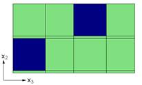
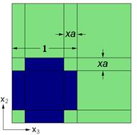
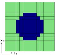
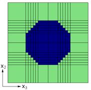
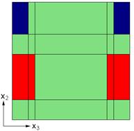
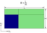
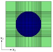
Figure 3.4 MAC/GMC 4.0 internal library of doubly periodic repeating unit cells (RUCs) without interface.



ARCHID = 1	ARCHID = 2

ARCHID = 3	ARCHID = 6

ARCHID = 9	ARCHID = 11

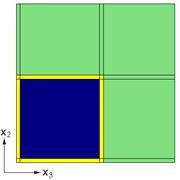
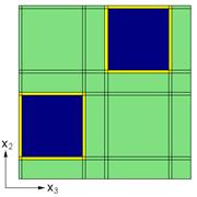
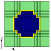
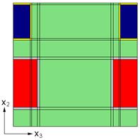
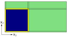
Figure 3.5 MAC/GMC 4.0 internal library of doubly periodic repeating unit cells (RUCs) with interface.


ARCHID = 0	ARCHID = 1

ARCHID = 2	ARCHID = 3

ARCHID = 4	ARCHID = 10

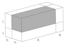
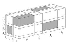
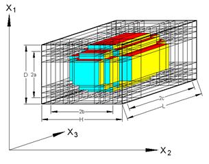
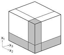
Figure 3.6 MAC/GMC 4.0 internal library of triply periodic repeating unit cells (RUCs).

Table 3.3 Constraints on the fiber volume fraction of the MAC/GMC 4.0 internal RUC architectures.

Doubly Periodic RUC Architectures
Architecture		Limit(s) on vf
0	Monolithic Material	–
1	Square Fiber, Square Pack
2	Square Fiber, Hexagonal Pack
3	Square Fiber, Square Diagonal Pack
4	Cross Shaped Fiber, Square Pack
6	7´7 Circular Fiber Approx., Rectangular Pack	R > 1 R < 1
7	14´14 Circular Fiber Approx., Rectangular Pack	R > 1 R < 1
9	Two Different Size Fibers, Rectangular Pack
11	Square Fiber, Rectangular Pack	for R > 1. for R < 1.
13	26´26 Circular Fiber Approx., Rectangular Pack	for R > 1. for R < 1.

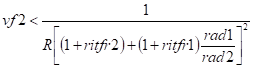
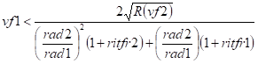
Table 3.3 (continued)

Triply Periodic RUC Architectures
0	Monolithic Material	–
1	Short Fibers in Square Array	vf < 1.
2	Short Fibers in Diagonal Array	for asp2 > asp1 for asp1 > asp2
3	Offset Short Fibers in Square Array
4	Ellipsoidal Inclusion, Rectangular Array	Analytical expressions unavailable
10	Open Cell ⁵	vf < 1.

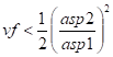
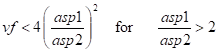
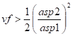
II. User-Defined Architecture (archid=99)

Usage:

*RUC

MOD=modid ARCHID=archid

NA=na NB=nb NG=ng

D=d(1),d(2),…,d(na)

H=h(1),h(2),…,h(nb)

L=l(1),l(2),…,l(ng)

SM=… ® specifics: see Table 3.4 ¬

Table 3.4 Format of the subcell material specification for user-defined RUC architectures.

Doubly Periodic RUC Analysis

Triply Periodic RUC Analysis

SM=m(nb,1),m(nb,2),…,m(nb,ng)

SM=m(nb-1,1),m(nb-1,2),…,m(nb-1,ng)

SM=m(1,1),m(1,2),…,m(1,ng)

(See Figure 3.7)

# -- gamma = 1

SM=m(na,1,1),m(na,2,1),…,m(na,nb,1)

SM=m(na-1,1,1),m(na-1,2,1),…,m(na-1,nb,1)

SM=m(1,1,1),m(1,2,1),…,m(1,nb,1)

# -- gamma = 2

SM=m(na,1,2),m(na,2,2),…,m(na,nb,2)

SM=m(na-1,1,2),m(na-1,2,2),…,m(na-1,nb,2)

SM=m(1,1,2),m(1,2,2),…,m(1,nb,2)

# -- gamma = ng

SM=m(na,1,ng),m(na,2,ng),…,m(na,nb,ng)

SM=m(na-1,1,ng),m(na-1,2,ng),…,m(na-1,nb,ng)

SM=m(1,1,ng),m(1,2,ng),…,m(1,nb,ng)

(See Figure 3.8)

Name	Definition
modid ^1,2	Periodic material model indentifier: = 1 ® monolithic material (internally uses doubly periodic GMC with one subcell) = 2 ® doubly periodic GMC model = 3 ® triply periodic GMC model = 12 ® doubly periodic HFGMC model
archid [=99]	I.D. number of RUC architecture (archid=99 for user-defined)
na ³	Number of subcells in the x₁-direction (Special Case) (see Figure 3.2)
nb	Number of subcells in the x₂-direction (see Figure 3.1 and Figure 3.2)
ng	Number of subcells in the x₃-direction (see Figure 3.1 and Figure 3.2)
d(1-na) ³	Subcell x₁-direction dimensions (Special Case) (see Figure 3.2)
h(1-nb)	Subcell x₂-direction dimensions (see Figure 3.1 and Figure 3.2)
l(1-ng)	Subcell x₃-direction dimensions (see Figure 3.1 and Figure 3.2)
specifics	This format depends on whether the RUC is doubly or triply periodic (see Table 3.4)
m(ib,ig)	Constituent material assigned to subcell b=ib g=ig (doubly-periodic case)
m(ia,ib,ig)	Constituent material assigned to subcell a=ig b=ib g=ig (triply-periodic case)

Examples:

Doubly Periodic

*RUC

MOD=2 ARCHID=99

NB=3 NG=3

H=0.5,0.5,1.0

L=0.5,1.0,0.5

SM=2,2,2

SM=2,2,3

SM=1,2,2

Figure 3.7 Example user-defined doubly periodic RUC.

Triply Periodic

*RUC

MOD=3 ARCHID=99

NA=4 NB=2 NG=2

D=1.,1.,1.,1.

H=1.,1.

L=1.,1.

# -- gamma = 1

SM=2,2

SM=1,2

# -- gamma = 2

SM=2,2

SM=1,1

SM=2,2

SM=1,2

Figure 3.8 Example user-defined Triply periodic RUC.

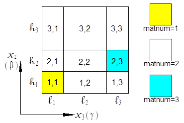
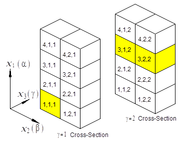
Associated MAC/GMC 4.0 Example Problem(s):

Example 3c, Example 3e, Example 5f, Example 7d, Example 7e

Notes:

1) modid=1 is a special case used in MAC/GMC 4.0 to select a monolithic material. Internally, the code employs a double periodic GMC RUC analysis with one subcell to which the material is assigned using M=mm (see Example above). A monolithic material may also be selected by using archid=0 in either doubly or triply periodic GMC.

2) Doubly periodic HFGMC RUC analysis requires an even number of subcells in both the x₂- and x₃-directions and additional specialized input under the *SOLVER keyword.

3) NA=na and D=d(1),d(2)…,d(na) are only required in the special case of triply periodic RUC analysis

Additional Information:

MAC/GMC 4.0 Keywords Manual Section 3 (*LAMINATE)

MAC/GMC 4.0 Theory Manual Section 2

*LAMINATE: Laminate analysis and architecture

P Either *RUC or *LAMINATE is required in all input files P

Purpose:

Invoke laminate analysis (as opposed to repeating unit cell analysis) for the problem, which requires selection of a micromechanics model as well as specification of an RUC architecture (i.e., arrangement of the composite constituents) for the analysis of each each ply. Lastly, the angle and thickness of each ply must be specified.

The *LAMINATE section is broken into two sub-sections:

I. Layer RUC Architecture from Internal Library (archid≠99)

II. User-Defined Layer RUC Architecture (archid=99)

I. Layer RUC Architecture from Internal Library (archid≠99)

Usage:

*LAMINATE

NLY=nly

LY=ly MOD=modid THK=thk ANG=ang ARCHID=archid &

® specifics: see Table 3.1 and Table 3.2 ¬ EM=em

® Repeated nly times

Name	Definition
nly	Number of layers (plies) comprising the laminate
ly	Layer number (data following LY=ly is associated with layer number ly)
modid ^1,2	Periodic material model indentifier: = 1 ® monolithic material (internally uses doubly periodic GMC with one subcell) = 2 ® doubly periodic GMC model = 3 ® triply periodic GMC model = 12 ® N/A (HFGMC unavailable within laminate)
thk	Thickness of layer
ang	Off-axis angle of layer (see Figure 3.3)
archid	I.D. number of RUC architecture (archid=99 for user-defined)
specifics³	This format depends on the modid and archid selected (see Table 3.1 and Table 3.2)
em ⁵	Electromagnetic specifier for layer number ly: = 1 ® Layer is electromagnetic = 0 ® Layer is not electromagnetic

Examples:

*LAMINATE

NLY=3

LY=1 MOD=2 THK=0.25 ANG=90 ARCHID=1 VF=0.65 F=1 M=2

LY=2 MOD=2 THK=0.50 ANG=0 ARCHID=1 VF=0.65 F=1 M=2

LY=3 MOD=2 THK=0.25 ANG=90 ARCHID=1 VF=0.65 F=1 M=2

*LAMINATE

NLY=4

LY=1 MOD=1 THK=0.25 M=2

LY=2 MOD=2 THK=0.25 ANG=60 ARCHID=6 R=1. VF=0.25 F=1 M=2

LY=3 MOD=3 THK=0.25 ANG=0 ARCHID=3 ASP1=3. ASP2=2. DR=1. &

VF=0.25 F=1 M=2

LY=4 MOD=3 THK=0.25 ANG=0. ARCHID=1 VF=0.25 ASP=1 F=1 M=2

Associated MAC/GMC 4.0 Example Problem(s):

Example 1b, Example 3g, Example 3h, Example 3i, Example 4d, Example 4e, Example 4g, Example 5c, Example 5d, Example 6c

Notes:

1) modid=1 is a special case used in MAC/GMC 4.0 to select a monolithic layer. Internally, the code employs a double periodic GMC RUC analysis for the layer with one subcell to which the material is assigned using M=mm (see Example above). A monolithic material may also be selected for a layer by using archid=0 in either doubly or triply periodic GMC.

2) The ability to employ triply periodic layers in a laminate is new to version 4.0 of the code. Doubly periodic HFGMC RUC analysis is not currently available for laminate layers.

3) Refer to the *RUC description earlier in this section of this manual for the specific input requirements for each RUC architecture. The RUC architectures contained within the MAC/GMC 4.0 architecture library are shown in Figure 3.4 (doubly periodic, no interface), Figure 3.5 (doubly periodic, with interface), and Figure 3.6 (triply periodic).

4) The ritfr and mi data is associated with the special case involving a layer with an RUC that has a separate interface material (see Figure 3.5). Only those RUCs shown in Figure 3.5 have the interface option available. To specify one of these RUCs with an interface for the layer, simply include the special case data shown in blue.

5) The electromagnetic specifier (EM=em) for the layer tells the code whether or not a particular layer is electromagnetically active. This is only required in the special case in which an electromagnetic analysis has been selected by including the *ELECROMAG keyword in the input file.

Additional Information:

MAC/GMC 4.0 Keywords Manual Section 3 (*RUC)

MAC/GMC 4.0 Theory Manual Section 3

II. User-Defined Layer RUC Architecture (archid=99)

Usage:

*LAMINATE

NLY=nly

LY=ly MOD=modid THK=thk ANG=ang ARCHID=archid EM=em &

MOD=modid ARCHID=archid

NA=na NB=nb NG=ng

D=d(1),d(2),…,d(na)

H=h(1),h(2),…,h(nb)

L=l(1),l(2),…,l(ng)

SM=… ® specifics: see Table 3.4 ¬

® Repeated nly times

Name	Definition
nly	Number of layers (plies) comprising the laminate
ly	Layer number (data following LY=ly is associated with layer number ly)
modid ^1,2	Periodic material model indentifier: = 1 ® monolithic material (internally uses doubly periodic GMC with one subcell) = 2 ® doubly periodic GMC model = 3 ® triply periodic GMC model = 12 ® N/A (HFGMC unavailable within laminate)
thk	Thickness of layer
ang	Off-axis angle (Figure 3.3) of layer
archid [=99]	I.D. number of RUC architecture (archid=99 for user-defined)
em ³	Electromagnetic specifier for layer number ly (Special Case): = 1 ® Layer is electromagnetic = 0 ® Layer is not electromagnetic
na ⁴	Number of subcells in the x₁-direction (Special Case) (see Figure 3.2)
nb	Number of subcells in the x₂-direction (see Figure 3.1 and Figure 3.2)
ng	Number of subcells in the x₃-direction (see Figure 3.1 and Figure 3.2)
d(1-na) ⁴	Subcell x₁-direction dimensions (Special Case) (see Figure 3.2)
h(1-nb)	Subcell x₂-direction dimensions (see Figure 3.1 and Figure 3.2)
l(1-ng)	Subcell x₃-direction dimensions (see Figure 3.1 and Figure 3.2)
specifics	This format depends on whether the RUC is doubly or triply periodic (see Table 3.4)
m(ib,ig)	Constituent material assigned to subcell b=ib g=ig (doubly-periodic case)
m(ia,ib,ig)	Constituent material assigned to subcell a=ig b=ib g=ig (triply-periodic case)

Examples:

*LAMINATE

NLY=2

LY=1 THK=0.5 ANG=0. MOD=2 ARCHID=99

NB=1 NG=2

H=1.

L=0.5,0.5

SM=1,2

LY=2 THK=0.5 ANG=90. MOD=2 ARCHID=1 VF=0.25 F=1 M=2

*LAMINATE

NLY=3

LY=1 THK=0.25 ANG=0. MOD=3 ARCHID=99 EM=1

NA=1 NB=2 NG=2

D=1.

H=0.5,0.5

L=0.5,0.5

SM=1,2

SM=2,2

LY=2 THK=0.5 ANG=90. MOD=2 ARCHID=1 VF=0.25 F=4 M=5 EM=0

LY=3 THK=0.25 ANG=0. MOD=3 ARCHID=99 EM=1

NA=1 NB=2 NG=2

D=1.

H=0.5,0.5

L=0.5,0.5

SM=1,2

SM=2,2

Associated MAC/GMC 4.0 Example Problem(s):

Example 7c

Notes:

2) Doubly periodic HFGMC RUC analysis is not currently available for laminate layers.

3) The electromagnetic specifier (EM=em) for the layer tells the code whether or not a particular layer is electromagnetically active. This is only required in the special case in which an electromagnetic analysis has been selected by including the *ELECROMAG keyword.

4) modid=NA and D=d(1),d(2)…,d(na) are only required in the special case of triply periodic RUC analysis.

Additional Information:

MAC/GMC 4.0 Keywords Manual Section 3 (*RUC)

MAC/GMC 4.0 Theory Manual Section 3

Section 4 : Loading Keywords

This section presents the four MAC/GMC 4.0 keywords that are related to the applied loading. These are:

*MECH ® Specify mechanical (and electromagnetic) loading profile

*THERM ® Specify thermal loading profile

*SOLVER ® Specify time-integration data

*SURF ® Specify loading (and additional information) for yield surface analysis

Because MAC/GMC 4.0 allows for inelastic material behavior, the simulated loading must be applied in an incremental manner. The problem solutions are (in general) path-dependent, so the overall solution (at the completion of the applied loading) actually involves solving the problem at each increment of the simulated applied loading. As such, a simulated loading profile must be specified rather than just the final load levels. The loading profile is essentially a load vs. time history that MAC/GMC 4.0 will apply to the specified RUC or laminate.

For repeating unit cell analysis, mechanical loading takes the form of an admissible time profile for each of the six global (stress or strain) components present in the RUC constitutive equation. For example, consider the standard (non-electromagnetic) repeating unit cell effective constitutive equation,

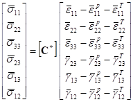
where are the global (or average) stress components on the composite, is the global (or effective) stiffness matrix, are the global (or average) normal strain components on the composite, are the global (or average) engineering shear strain components on the composite, are the global (or average) normal inelastic strain components on the composite, are the global (or average) engineering shear inelastic strain components on the composite, are the global (or average) normal thermal strain components on the composite, and are the global (or average) engineering shear thermal strain components on the composite. Admissibility simply requires that, if a particular strain component is specified, the corresponding stress component cannot be specified (and vice versa). In addition to the arbitrary mechanical loading option (which allows the user to specify all six loading components, MAC/GMC 4.0 also includes several internal loading options that simplify the application of loading for commonly used mechanical loading types. In the special case of electromagnetic RUC analysis, the number of loading components is increased from six to twelve to accommodate applied electric and magnetic load components (see the MAC/GMC 4.0 Theory Manual Section 2.1.2).

The applied mechanical loading for laminate analysis is different than that of RUC analysis. Globally, rather than dealing with average stresses and strains, the applicable quantities are stress and moment resultants along with midplane strains and curvatures (see the MAC/GMC 4.0 Theory Manual Section 3). For laminate analysis, the code’s internal mechanical loading options are numbered differently than those associated with RUC mechanical loading. As is the case in electromagnetic RUC analysis, electromagnetic laminate analysis involves additional electromagnetic loading components.

MAC/GMC 4.0 also allows application of a simulated time vs. temperature profile for both RUC and laminate analysis using the *THERM keyword. It should be noted that the temperature at every point in time is treated as constant throughout the RUC or laminate; the code does not solve any thermal boundary value problems, but rather treats the temperature history as known. The *SOLVER keyword is used to select either a constant time step forward Euler time integration scheme, or a self-adaptive predictor-corrector time integration scheme. Finally, the yield surface option keyword (*SURF) is a special case in that the yield surface “probing” (i.e., loading along different angles in a particular stress space) controls the applied loading. In this case, the data specified under *MECH, *THERM, and *SOLVER are considered to be a “preload” that occurs before the start of the yield surface analysis.

*MECH: Applied mechanical loading

Purpose:

Specify the simulated mechanical (and electromagnetic) loading profile for the RUC or laminate.

Usage:

*MECH

LOP=lop REFTIME=reftime

NPT=npt TI=t(1),t(2),…,t(npt) MAG=mag(1),mag(2),…,mag(npt) &

MODE=mode(1),mode(2),…,mode(npt-1)

® Repeated number of times equal to number of specified load components (see Table 4.1)

Name	Definition
lop ¹	Loading option (see Table 4.1) (lop = 99 ® arbitrary mechanical loading option)
reftime ²	Strain reference time (Optional)
npt	Number of time vs. load magnitude points in specified profile
t(i) ³	Time points in time vs. load magnitude profile (see Figure 4.1)
mag(i) ^4,5	Load magnitude points in time vs. load magnitude profile (see Figure 4.1)
mode(j) ⁶	Mode of applied loading during loading step from t(j) to t(j+1) = 1 ® strain, midplane strain, electric field, magnetic field applied = 2 ® stress, force resultant, electric displacement, magnetic flux density applied

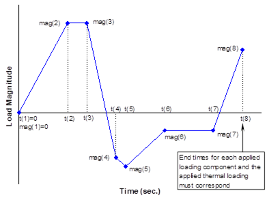
Figure 4.1 Example time vs. load magnitude profile for an applied loading component.

Examples:

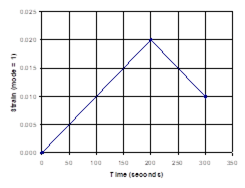
*MECH

LOP=1

NPT=3 TI=0.,200.,300. MAG=0.,0.02,0.01 MODE=1,1

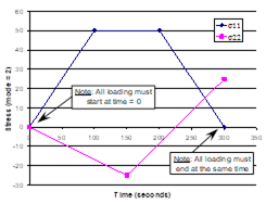
*MECH

LOP=7

NPT=4 TI=0.,100.,200.,300. MAG=0.,50.,50.,0. MODE=2,2

NPT=3 TI=0.,150.,300. MAG=0.,-25.,25. MODE=2,2

*MECH

LOP=99

NPT=6 TI=0.,300.,310.,2310.,2320.,2620. MAG=0.,0.,0.01,0.01,0.,0. &

MODE=1,1,1,2,2

NPT=6 TI=0.,300.,310.,2310.,2320.,2620. MAG=0.,0.,0.005,0.005,0.,0. &

MODE=1,1,1,2,2

NPT=2 TI=0.,2620. MAG=0.,0. MODE=2

NPT=6 TI=0.,300.,310.,2310.,2320.,2620. &

MAG=0.,0.,0.0075,0.0075,0.,0. MODE=1,1,1,2,2

*MECH

LOP=99

NPT=2 TI=0.,600. MAG=0.,0. MODE=2

NPT=2 TI=0.,600. MAG=0.,0. MODE=1

NPT=2 TI=0.,600. MAG=0.,6.E6 MODE=1

Table 4.1 MAC/GMC 4.0 loading options for doubly and triply periodic RUC and laminate analysis.

*lop*	number components specified	Doubly Periodic RUC Analysis		Triply Periodic RUC Analysis		Laminate Analysis
		mode = 1	mode = 2	mode = 1	mode = 2	mode = 1	mode = 2
1	1	e₁₁	s₁₁	e₁₁	s₁₁		N_xx
2	1	e₂₂	s₂₂	e₂₂	s₂₂		N_yy
3	1	e₃₃	s₃₃	e₃₃	s₃₃		N_xy
4	1	g₂₃	s₂₃	g₂₃	s₂₃	κ_xx	M_xx
5	1	g₁₃	s₁₃	g₁₃	s₁₃	κ_yy	M_yy
6	1	g₁₃	s₁₂	g₁₃	s₁₂	κ_xy	M_xy
7	2	e₁₁ & e₂₂	s₁₁ & s₂₂	e₁₁ & e₂₂	s₁₁ & s₂₂	N/A
8	2	e₂₂ & e₃₃	s₂₂ & s₃₃	e₂₂ & e₃₃	s₂₂ & s₃₃	N/A
9	2	e₁₁ & g₂₃	s₁₁ & s₂₃	e₁₁ & e₃₃	s₁₁ & s₃₃	N/A
10	2	e₂₂ & g₁₃	s₂₂ & s₁₃	e₁₁ & g₂₃	s₁₁ & s₂₃	N/A
11	2	N/A		e₂₂ & g₁₃	s₂₂ & s₁₃	N/A
12	2	N/A		e₃₃ & g₁₂	s₃₃ & s₁₂	N/A
99	6	6 of e_ij or s_ij		6 of e_ij or s_ij		3 of or N_ij, 3 of or M_ij
99	12 (electromag)	6 of e_ij or s_ij, 3 of E_k or D_k, 3 of H_k or B_k		6 of e_ij or s_ij, 3 of E_k or D_k, 3 of H_k or B_k		3 of or N_ij, 3 of or M_ij, 3 of E_k, 3 of H_k

F Note: s_ij = stress, e_ij = normal strain, g_ij = engineering shear strain, N_ij = force resultant, M_ij = moment resultant, = midplane strains, κ_ij = midplane curvatures, D_k = electrical displacements, E_k = electric fields, B_k = magnetic flux densities, H_k = magnetic fields.

Associated MAC/GMC 4.0 Example Problem(s):

Example 1c-d, Example 2a-h, Example 3a-i, Example 4a, Example 4b, Example 4c, Example 4d, Example 4e, Example 5b-f, Example 6a-b, Example 7a, Example 7b, Example 7c

Notes:

1) As shown in Table 4.1, certain values of lop are invalid in certain cases. In particular, lop=11 and lop=12 are only valid for triply periodic RUC analysis, while for laminate analysis, the only valid values for lop are 1–6 and 99.

2) The optional REFTIME=reftime specifier is used to set a reference strain value other than zero. The reference strain is the strain value that all the rest of the specified loading strain values are taken with respect to. For example, if the reference strain were 0.015, and a strain load of 0.01 were specified, the code would increase the strain to 0.025. Instead of specifying the reference strain directly, a time is given at which the strain state is taken as the six reference strain components. This feature is useful when simulating residual stresses prior to applying loading in the form of strains (see MAC/GMC 4.0 Example Problem 4b).

3) The first time specified for each mechanical (and electromagnetic) loading component must be zero, and the final time for each component must be the same. However, the number of intermediate times, as well as the intermediate times themselves, can be different for each applied loading component.

4) The units of the applied loading should be consistent with the units employed for the constituent materials. That is, for example, if the units of the constituent material elastic moduli are MPa, any applied stress components will be interpreted by the code as having the units MPa.

5) The first specified load magnitude should be zero. The code must begin its execution in an unloaded state.

6) In the special case of an electromagnetically active laminate, the electromagnetic loading currently can only take the form of applied electric field components (E_k) and magnetic field (H_k) components. That is, laminate electric displacement (D_k) and magnetic flux density (B_k) components cannot currently be applied.

Additional Information:

MAC/GMC 4.0 Keywords Manual Section 1 (*ELECTROMAG)

MAC/GMC 4.0 Theory Manual Sections 2 and 3

*THERM: Applied thermal loading

Purpose:

Specify the simulated thermal loading profile (time vs. temperature) for the RUC or laminate.

Usage:

*THERM

NPT=npt TI=t(1),t(2),…,t(npt) TEMP=T(1),T(2),…,T(npt)

Name	Definition
npt	Number of time vs. temperature points in specified profile
t(i) ¹	Time points in time vs. temperature profile (see Figure 4.2)
T(i) ²	Temperature points in time vs. load temperature profile (see Figure 4.2)

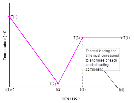
Figure 4.2 Example temperature vs. time profile for applied thermal loading.

Example:

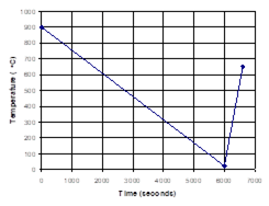
*THERM

NPT=3 TI=0.,6000.,6600. TEMP=900.,23.,650.

Associated MAC/GMC 4.0 Example Problem(s):

Example 1d, Example 2e-h, Example 3a-i, Example 4a, Example 4b, Example 4c, Example 4d, Example 4e, Example 5b-f, Example 6a-b, Example 7a-c

Note:

1) The starting time for the time vs. temperature profile must be zero. The ending time for the time vs. temperature profile must correspond to the ending time for any specified mechanical loading.

2) The temperature unit in MAC/GMC 4.0 is °C. The user may employ other temperature units if none of the constituent materials are taken from the code’s internal material database.

Additional Information:

MAC/GMC 4.0 Theory Manual Sections 2 and 3

*SOLVER: Time integration

Purpose:

Allows specification of time integration scheme and associated integration related data.

Only two choices are currently available, thus the *SOLVER section is broken into two corresponding sub-sections:

I. Forward Euler Time Integration (specified time step) (method=1)

II. Predictor-Corrector Time Integration (self-adaptive time step) (method=2)

I. Forward Euler Time Integration (method=1)

Usage:

*SOLVER

METHOD=method NPT=npt TI=t(1),t(2),…,t(npt) STP=stp(1),stp(2),…,stp(npt-1) &

ITMAX=itmax ERR=errtol

NLEG=nleg NINTEG=nint

Name	Definition
method [=1]	Time integration method: = 1 ® Forward Euler (specified time step) = 2 ® Predictor-Corrector (self-adaptive time-step)
npt	Number of time vs. step size points in specified profile
t(i) ¹	Time points in time vs. step size profile
stp(i) ²	Step sizes in time vs. step size profile
itmax ³	Maximum number of global equilibrium iterations (Special Case)
errtol ³	Error tolerance for convergence of global iterations (Special Case)
nleg ^4,5	Order of the Legendre polynomial used to approximate the inelastic strain field (Special Case)
nint ^4,5	Number of integration points used to represent the field variables (Special Case)

Examples:

*SOLVER

METHOD=1 NPT=4 TI=0.,60.,180.,240. STP=0.1,0.5,0.2

*SOLVER

METHOD=1 NPT=2 TI=0.,20. STP=0.1 ITMAX=20 ERR=0.0001

NLEG=5 NINTEG=11

Associated MAC/GMC 4.0 Example Problem(s):

Example 1c-d, Example 2a-h, Example 3a-i, Example 4a-f, Example 5b-f, Example 6a-c, Example 7a-c

Note:

1) The starting time in the time vs. step size profile must be zero. The ending time must correspond to the ending time of any mechanical and thermal loading specified under *MECH and *THERM. The ending time must correspond to the ending time of any mechanical and thermal loading specified under *MECH and *THERM.

2) The forward Euler integration scheme involves stepping through time with a specified time step size. At each time step, increments of the field variables throughout the RUC or laminate are calculated and simply added to the previous field variable values. The user specifies a number of time points along with the time step size to be used between each successive time point (see Example above). If the time step is too large, the time integration can diverge, which leads to oscillations or overflow in the results (see Example Problem 7a). The maximum permissible time step size that still allows convergence is problem dependent; users are encouraged to experiment with this value for their problems of interest.

3) ITMAX=itmax and ERR=errtol are required only in the special case when one or more constituent material is modeled a) using classical incremental plasticity (cmod=21) or b) implicit multimechanism GVIPS (cmod=22). These two constitutive models require iterations (at each increment of the applied loading) to ensure that global equilibrium is satisfied.

a) In the case of incremental plasticity, to quantify convergence of the global iterations, MAC/GMC 4.0 employs the local effective plastic strain increment as a measure of the error. Convergence is achieved when the fractional change of the effective plastic strain increment from one iteration to the next is less than errtol throughout the RUC or laminate.

b) In the case of implicit multimechanism GVIPS, a global energy related increment is employed as a measure of error. Convergence is achieved when the fractional change of this increment from one iteration to the next is less than errtol. The acceptable value of errtol is problem dependent. Users are encouraged to experiment with this value for their specific problems of interest. Note that this constitutive model employs a local implicit integration scheme internally.

4) NLEG=nleg and NINTEG=nint are required only in the special case of doubly periodic RUC analysis using HFGMC (modid=12). In this case, the inelastic strain field can vary arbitrarily throughout the RUC. In order to represent the inelastic strain field in HFGMC, MAC/GMC 4.0 employs Legendre polynomials, the order of which must be specified. In addition, the number of integration points at which all field variables are tracked must be specified. nint is the number of integration points for both the x₂- and x₃-directions per subcell. Thus, for example, if NINTEG=11 is specified, 11 integration points are used per subcell in each of the two direction, for a total of 121 integration points for each subcell.

5) The values NLEG=5 and NINTEG=11 have been shown to yield good precision in the local fields predicted by HFGMC. These values should be employed as default values unless the user is confident in using other values.

Additional Information:

MAC/GMC 4.0 Keywords Manual Section 2 (*CONSTITUENTS)

MAC/GMC 4.0 Keywords Manual Section 3 (*RUC)

MAC/GMC 4.0 Theory Manual Section 7.1

II. Predictor-Corrector Time Integration (method=2)

Usage:

*SOLVER

METHOD=method ISTM=istm ISTT=istt ERR=errtol MINSTEP=minstp

Name	Definition
method [=2] ¹	Time integration method: = 1 ® Forward Euler (specified time step) = 2 ® Predictor-Corrector (self-adaptive time-step)
istm ²	Initial mechanical loading time step
istt ²	Initial thermal loading time step
errtol ³	Error tolerance for time step size changes
minstp⁴	Minimum time step size

Example:

*SOLVER

METHOD=2 ISTM=0.001 ISTT=0.1 ERR=0.001 MINSTEP=0.00001

Associated MAC/GMC 4.0 Example Problem(s):

Example 4h

Notes:

1) The self-adaptive predictor-corrector integration scheme cannot currently be utilized in conjunction with the following features:

a) Laminate analysis (*LAMINATE)

b) Fatigue damage analysis (*DAMAGE)

c) Classical incremental plasticity (cmod=21)

d) Implicit multimechanism GVIPS (cmod=22).

2) The self-adaptive predictor-corrector integration scheme employs a fourth-order Runge-Kutta starter, an Adams-Bashforth four-step predictor, and an Adams-Moulton four step corrector (see the MAC/GMC 4.0 Theory Manual Section 7.2). It starts with a small time step that is permitted to increase, provided the error remains within acceptable limits. ISTM=istm and ISTT=istt are used to specify the initial (starting) time step sizes for mechanical and thermal loading. These are independent variables because the time scale is often vastly different for mechanical and thermal loading. The code chooses the appropriate initial time step size from istm and istt based on whether the initial applied loading (specified under *MECH and *THERM) involves any change in the mechanical or thermal load levels. If the mechanical and thermal load levels are both initially changing, the code will choose the smaller of istm and istt.

3) ERR=errtol specifies the acceptable fractional difference between predicted and corrected values of the field variables. If the fractional difference between these values for any field variable in any subcell is greater than errtol, the time step size will be cut in half. Otherwise, the time step size will be permitted to double, provided the history of each field variable required for prediction using the larger time step has been stored. An errtol value of 0.001 can be used as starting point, but an acceptable value can be problem dependent. Users are encouraged to experiment with this value for their problems of interest.

4) MINSTEP=minstp is used to prevent the time step from becoming too small. In some cases changing minstep to a larger value can significantly decrease execution time (i.e., speed up the execution) without compromising the accuracy of the code’s results.

Additional Information:

MAC/GMC 4.0 Keywords Manual Section 2 (*CONSTITUENTS)

MAC/GMC 4.0 Keywords Manual Section 3 (*RUC)

MAC/GMC 4.0 Theory Manual Section 7.2

*SURF: Yield Surface Analysis

Purpose:

Generate RUC or laminate yield surfaces.

Usage:

*SURF

TMAX=tmax STP=stp MMAX=mmax MODE=mode TREF=tref

OPTION=o₁,o₂,o₃,o₄,o₅,o₆,o₇

ISPX=ispx(1),ispx(2),ispx(3) ISPY=ispy(1),ispy(2),ispy(3) ANGINC=anginc

EPS=eps DR=dr ISR=isr IP=ip

Name	Definition
tmax ¹	Ending time for each probing excursion
stp ¹	Time step size for yield surface probing
mmax ¹	Ending load magnitude for each probing excursion
mode ¹	Mode of applied loading during yield surface probing = 1 ® strain or midplane strain applied = 2 ® stress or force resultant applied
tref ²	Reference temperature at which to generate yield surface (Special Case)
o₁ – o₇ ³	Yield surface generation options ® up to 7 specified (see Table 4.2) (Special Case)
ispx(1) ⁴	Controlling component for yield surface x-axis
ispx(2), ⁴ ispx(3)	Slave components to controlling x-axis component (Optional)
ispy(1) ⁴	Controlling component for yield surface y-axis
ispy(2), ⁴ ispy(3)	Slave components to controlling y-axis component (Optional)
anginc	Angle increment in stress space for yield surface probing
eps	Yield value for surface of equivalent plastic strain
dr	Yield value for surface of constant dissipation rate
isr	Yield value for surface of constant inelastic strain rate
ip	Yield value for surface of constant inelastic power

Example:

*SURF

TMAX=400. STP=0.01 MMAX=0.04 MODE=1 TREF=650.

OPTION=1,2,3,4

ISPX=1 ISPY=2,3 ANGINC=5.

EPS=0.0001 DR=0.00025 ISR=0.00002 IP=0.001

Associated MAC/GMC 4.0 Example Problem(s):

Example 4f, Example 4g

Notes:

1) MAC/GMC 4.0 generates yield surfaces by “probing” in a particular stress space until all yield criteria are satisfied. Probing involves applying multi-axial loading such that the angle in the specified stress space remains constant. For example, if the s₁₁-s₂₂ stress space were specified, probing at an angle of 45° would involve incremental application of s₁₁ = s₂₂ until all yield criteria were satisfied. Probing at an angle of 30° would involve application of s₂₂ = s₁₁ tan(30°) until all yield criteria were satisfied. When all angles from 0° to 360° are probed and the stresses at which yield is detected are recorded, the yield surface can be plotted from the data files generated by the code.

The loading for yield surface analysis is controlled under the *SURF keyword. This loading must be isothermal and always employs the forward Euler time integration scheme. In addition, the loading cannot be divided into separate portions with different time step sizes. Any loading information that is specified using *MECH, *THERM, and *SOLVER is treated as a “preload”. This preload is applied prior to the start of the yield surface probing and thus can be used to generate yield surfaces that incorporate residual stresses. tmax and mmax are the time and load magnitude at which yield surface probing will stop regardless of whether or not all yield surface criteria have been satisfied. Thus, if the code reaches this loading end point at a particular probing angle, the yield surface data for one or more plots will not be valid at this angle, and a warning will be written to the output file. It is therefore desirable to make the loading end point large so that yielding can always occur before the end point is reached. The code automatically stops probing at a particular angle when all yield criteria are satisfied, so employing large tmax and mmax values will not adversely affect execution time.

Note that in order to generalize the specified loading for the multi-axial loading required for yield surface probing, the specified loading (mmax) is interpreted as an invariant quantity. In particular, for stress and force resultant control, mmax is interpreted as , while for strain control mmax is interpreted as . This allows the loading to be applied at a constant equivalent rate, regardless of probing angle.

2) TREF=tref is required in the special case that no thermal preloading has been specified. If thermal preloading is specified (using *THERM), the code assumes that the yield surface probing occurs at the ending temperature of the thermal preload. In the absence of thermal preloading, the code requires tref to specify the temperature for yield surface probing.

3) The yield surface options are given in Table 4.2. At least one option must be specified and up to four may be specified for RUC yield surface analysis. For laminate yield surfaces, up to seven options may be specified. Each yield surface option specified will cause a data file to be generated. This data file will contain the probing angle and the global stress state at which yielding was detected at that probing angle for each of the four yield surface types (eps, dr, isr, ip). In the case of OPTION=4 or OPTION=7, all of this data will be repeated for each individual ply or each individual subcell. Note that elastic subcells will be skipped.

4) The x and y stress space specifiers (ispx(j), ispy(j)) are used indicate to the code which loading components will be applied to generate the yield surface. ispx(1) and ispy(1 )are required. These are the controlling components that will occupy the x- and y- axes on the plot of the yield surface. Two optional slave components (ispx(2), ispx(3), ispy(2), ispy(3)) may be specified for each of the controlling components. The slave components will be loaded to the same value as the corresponding controlling components. For example, if s₁₁ and s₂₂ were specified as the x and y controlling components and s₃₃ were specified as a slave y component (ISPX=1 ISPY=2,3), at a probing angle of 30°, s₃₃ = s₂₂ = s₁₁ tan(30°) would be incrementally applied.

Note that for laminate yield surfaces, ispx(i) and ispy(i) can only take the values 1, 2, or 3, corresponding to in-plane loading. Thus, at most one slave component can be specified. Further, the yield surface analysis is only valid for symmetric laminates with no bending.

Table 4.2 Yield surface options (specified as OPTION=o_i) and output file names for RUC and laminate analyses.

o_i

RUC analysis

Laminate analysis

surface generated

file generated

surface

generated

file generated

RUC level global yield surface

surf_global.dat

Laminate level global yield surface

surf_global.dat

First subcell yield surface

surf_1st.dat

First ply yield surface

surf_1st_ply.dat

All subcells yield surface

surf_all.dat

All plies yield surface

surf_all_plies.dat

Yield surface for each individual subcell

surf_local.dat

Yield surface for each individual ply

surf_plies.dat

N/A

First subcell yield surface

surf_1st.dat

N/A

All subcells yield surface

surf_all.dat

N/A

Yield surface for each individual subcell

surf_local.dat

Additional Information:

MAC/GMC 4.0 Theory Manual Section 6

Section 5 : Damage and Failure Keywords

This section deals with the six MAC/GMC 4.0 keywords that enable analysis of damage and failure in composites materials and laminates. These are:

*ALLOWABLES ® Elastic estimation of the composite allowables

*FAILURE_SUBCELL ® Subcell level static failure analysis

*FAILURE_CELL ® RUC level static failure analysis

*DAMAGE ® Cyclic fatigue damage analysis

*DEBOND ® Internal fiber-matrix interfacial debonding

*CURTIN ® Curtin effective fiber breakage model for longitudinal fiber failure

Elastic allowables estimation is the simplest form of failure analysis available in MAC/GMC 4.0. Composite (RUC) allowable stress components are estimated based on the global level of each individual stress component that causes the allowable stress in a constituent material to be met. The composite allowable strain components are similarly estimated. These calculations are easily performed via the GMC concentration equations and are independent of any simulated loading applied to the composite. As such, the estimated allowables are like material properties for the specified RUC because altering the applied loading (e.g., adding simulated residual stresses) does not have an effect.

Static failure analysis within MAC/GMC 4.0 (via the *FAILURE_SUBCELL and *FAILURE_CELL keywords) is completely different from the allowables estimation. The static failure analysis monitors the stress and strain components in the composite or laminate (on the subcell or RUC level) and checks for failures using the specified failure criteria. Thus, the static failure analysis (like an actual experimental test) is inherently linked to the loading applied to the RUC or laminate and the predicted failure stress and strain are not truly material properties. That is, for example, a uni-axial tensile test on a highly strain rate dependent metallic alloy performed at a strain rate of 10^-2 per second would result in a completely different measured strength than that resulting from the same test on the same alloy performed at a strain rate of 10^-6 per second. Clearly, the strength measured for this material is not a material property, but is linked to the loading conditions to which the material is subjected. Static failure analysis within MAC/GMC 4.0 is the same way. The allowables estimation is a quick and simple first pass at predicting composite failure stresses and strains from the constituent allowables. For more realistic failure analyses, the static failure capabilities within MAC/GMC 4.0 should be employed.

The final three keywords covered in this section deal with more specialized damage and failure analysis techniques. *DAMAGE enables use of a simple strength reduction model (typically applied to the fiber constituent) and a more complex stiffness reduction model (typically applied to the matrix constituent) for composites and laminates subjected to cyclic loading. *DEBOND allows the effect of local fiber-matrix debonding, which is prevalent in some composites (most notably titanium matrix composites), to be included within RUC and laminate analyses. Finally, the Curtin effective fiber breakage model (*CURTIN) is an approach based on fiber strength statistics that account for the longitudinal stiffness reduction due to failure of fibers in RUCs and laminates.

*ALLOWABLES: Estimated elastic allowables

N Caution N

These estimated allowables should not be considered “design allowables”, which by definition have been extensively validated with experimental data

Purpose:

Estimate the composite allowables based on the allowables of the constituent materials and linear elastic concentration calculations. MAC/GMC 4.0 calculates three sets of elastic stress and strain allowable components, listed in order from most to least conservative:

1) First Subcell Allowables ® Global stress/strain at which the first subcell reaches its allowable stress/strain level

2) Average Material Allowables ® Global stress/strain at which the average material stress/strain for one of the constituents reaches its allowable stress/strain level

3) All Subcells Allowables ® Global stress/strain at which all of the subcells have reached their allowable stress/strain levels

Each allowable component is estimated based purely on a linear elastic concentration calculation involving application of a single global stress or strain component. Three separate sets of allowables are provided, an upper bound (all subcells allowables), lower bound (first subcell allowables), and an intermediate set (average material allowables), thus enabling the user to make a judicious choice based on the specific problem of interest. Note that the allowables estimation is available for RUC analysis only (not laminate analysis).

Usage:

*ALLOWABLES

NMAT=nmat

MAT=matnum

S11=s11 S22=s22 S33=s33 S23=s23 S13=s13 S12=s12 COMPR=comprs &

SC11=sc11 SC22=sc22 SC33=sc33

E11=e11 E22=e22 E33=e33 E23=e23 E13=e13 E12=e12 COMPR=compre &

EC11=ec11 EC22=ec22 EC33=ec33

® Repeated nmat times

Name	Definition
nmat	Number of constituent materials for which allowables are specified
matnum ¹	Material number of constituent whose allowables are being specified
s11, s22, s33 ²	Tensile normal stress allowables for material number matnum
s23, s13, s12 ²	Shear stress allowables for material number matnum
comprs	Compressive normal stress allowable specifier for material number matnum: = DIF ® Compressive stress allowables are different than tensile and must be specified = SAM ® Compressive stress allowables are the same as tensile should not be specified = OFF ® Do not utilize compressive stress allowables, and they should not be specified
sc11, sc22, sc33 ^2,3	Compressive normal stress allowables (Special Case)
e11, e22, e33 ²	Tensile normal strain allowables for material number matnum
e23, e13, e12 ^2,3	Shear strain allowables for material number matnum
compre	Compressive normal strain allowable specifier for material number matnum: = DIF ® Compressive strain allowables are different than tensile and must be specified = SAM ® Compressive strain allowables are the same as tensile should not be specified = OFF ® Do not utilize compressive strain allowables, and they should not be specified
ec11, ec22, ec33 ^2,4	Compressive normal strain allowables (Special Case)

Examples:

*ALLOWABLES

NMAT=2

MAT=1

S11=3500. S22=91.2 S33=91.2 S23=31.4 S13=134 S12=134. COMPR=SAM

E11=0.009 E22=0.012 E33=0.012 E23=0.012 E13=0.009 E12=0.009 COMPR=SAM

MAT=2

S11=80. S22=80. S33=80. S23=40. S13=40. S12=40. COMPR=SAM

E11=0.023 E22=0.023 E33=0.023 E23=0.031 E13=0.031 E12=0.031 COMPR=SAM

*ALLOWABLES

NMAT=1

MAT=3

S11=2500. S12=500. COMPR=OFF

E11=0.01 E22=0.012 E33=0.012 E23=0.012 E13=0.009 E12=0.01 COMPR=DIF &

EC11=0.005

Associated MAC/GMC 4.0 Example Problem(s):

Example 5a, Example 5b

Notes:

1) If a constituent material that is present in the RUC does not have allowables specified, the subcells that contain this material will not be considered in the allowables estimation. In such a case, the All Subcells Allowables will still be calculated by skipping the subcells containing the material in question.

2) If a particular component is omitted from either the stress or strain allowables input for a particular material, that component will not be considered in the calculation for subcells containing that particular material. If none of the materials within the RUC have an allowable specified for a particular component, an allowable will not be calculated for that component.

3) The specified shear strain allowables are interpreted by the code as engineering shear strains.

4) The compressive stress and strain allowables (sc11, sc22, sc33, ec11, ec22, ec33) are only required in the special case when the compression specifier (comprs or compre) =DIF. Otherwise, the compressive stress and strain allowables should be omitted.

Additional Information:

MAC/GMC 4.0 Theory Manual Section 5.1

*FAILURE_SUBCELL: Subcell static failure

Purpose:

Perform static failure analysis based on the local stress and strain fields in the subcells. Static failure analysis involves checking the specified failure criteria during application of a simulated thermo-mechanical loading history. This is distinct from the allowables estimation, which is a linear elastic concentration calculation independent of the applied loading and any material history dependence. Thus, while the allowables may be considered predicted material properties for a composite, the static failure predictions are inherently linked to the specifics of the simulated loading applied to the composite. The maximum stress, maximum strain, and Tsai-Hill failure criteria are available within MAC/GMC 4.0. This availability, however, does not imply endorsement of these criteria by any parties associated with the code. The static failure analysis capabilities should be used with caution.

Usage:

*FAILURE_SUBCELL

NMAT=nmat

MAT=matnum NCRIT=ncrit

CRIT=crit X11=x11 X22=x22 X33=x33 X23=x23 X13=x13 X12=x12 COMPR=compr &

XC11=xc11 XC22=xc22 XC33=xc33 ACTION=action

® Repeated ncrit times

® Repeated nmat times

Name	Definition
nmat	Number of constituent materials for which failure parameters are specified
matnum ¹	Material number of constituent whose failure parameters are being specified
ncrit	Number of failure criteria to check for material number matnum
crit	Failure criterion material number matnum: = 1 ® Maximum stress failure criterion = 2 ® Maximum strain failure criterion = 3 ® Tsai-Hill multi-axial failure criterion
x11, x22, x33 ²	Tensile normal failure parameters for material number matnum and criterion number crit (failure stresses for crit=1, or 3, failure strains for crit=2)
x23, x13, x12 ^2,3	Shear failure parameters for material number matnum and criterion number crit (failure stresses for crit=1, or 3, failure strains for crit=2)
compr	Compressive normal failure specifier for material number matnum and criterion number crit: = DIF ® Compressive parameters are different than tensile and must be specified = SAM ® Compressive parameters are the same as tensile should not be specified = OFF ® Do not utilize compressive parameters, and they should not be specified

Name

Definition

xc11, xc22, xc33 ^2,4

Compressive normal failure parameters for material number matnum and criterion number crit (failure stresses for crit=1, or 3, failure strains for crit=2)

(Special Case)

action ⁵

Action for code to take upon detection of subcell failure:

= 1 ® Zero subcell stiffness and continue execution

= 0 ® Do nothing and continue (write notification to output file)

= -1 ® Stop execution

Examples:

*FAILURE_SUBCELL

NMAT=2

MAT=1 NCRIT=2

CRIT=1 X11=3500. X22=91.2 X33=91.2 X23=31.4 X13=134. X12=134. &

COMPR=OFF ACTION=1

CRIT=2 X11=0.009 X22=0.012 X33=0.012 X23=0.012 X13=0.009 X12=0.009 &

COMPR=OFF ACTION=1

MAT=2 NCRIT=2

CRIT=1 X11=80. X22=80. X33=80. X23=40. X13=40. X12=40. &

COMPR=OFF ACTION=1

CRIT=2 X11=0.023 X22=0.023 X33=0.023 X23=0.031 X13=0.031 X12=0.031 &

COMPR=OFF ACTION=1

*FAILURE_SUBCELL

NMAT=2

MAT=4 NCRIT=1

CRIT=3 X11=3500. X22=91.2 X33=91.2 X23=31.4 X13=134. X12=134. &

ACTION=-1

MAT=7 NCRIT=2

CRIT=1 X22=80. X33=80. X23=40. COMPR=DIF &

XC22=100. XC33=100. XC23=60. ACTION=0

CRIT=2 X11=0.023 COMPR=SAM ACTION=1

Associated MAC/GMC 4.0 Example Problem(s):

Example 5b, Example 5c, Example 5d

Notes:

1) If a constituent material that is present in the RUC does not have subcell failure parameters specified, the subcells that contain this material will not be considered when checking for failure (i.e., they are treated as infinitely strong).

2) If a particular component (xij) is omitted from the failure parameters for either the maximum stress or maximum strain criterion, that component will not be considered when checking for failure of subcells containing that particular material. For the Tsai-Hill criterion, all of the components (xij) are required.

3) In the case of the maximum strain criterion, the specified shear failure strains are interpreted by the code as engineering shear strains.

4) The compression specifier (compr) and the compressive failure parameters (xc11, xc22, xc33) are not required for the Tsai-Hill criterion. The compressive failure parameters (xc11, xc22, xc33) are only required for the maximum stress and maximum strain criteria in the special case when the compression specifier compr=DIF. Otherwise, the compressive failure parameters should be omitted.

5) ACTION=action is ignored in the case of fatigue damage analysis (*DAMAGE) and can be omitted in that case.

Additional Information:

MAC/GMC 4.0 Theory Manual Section 5.2

*FAILURE_CELL: Repeating unit cell static failure

Purpose:

Perform static failure analysis based on the RUC level stress and strain fields. As with subcell level static failure analysis, RUC level static failure analysis involves checking the specified failure criteria during application of a simulated thermo-mechanical loading history. Thus, the RUC level static failure predictions are inherently linked to the specifics of the simulated loading applied to the composite.

Usage:

*FAILURE_CELL

NCRIT=ncrit

CRIT=crit X11=x11 X22=x22 X33=x33 X23=x23 X13=x13 X12=x12 COMPR=compr &

XC11=xc11 XC22=xc22 XC33=xc33 ACTION=action

® Repeated ncrit times

Name	Definition
ncrit	Number of RUC level failure criteria to check
crit	Failure criterion: = 1 ® Maximum stress failure criterion = 2 ® Maximum strain failure criterion = 3 ® Tsai-Hill multi-axial failure criterion
x11, x22, x33 ¹	Tensile normal failure parameters for criterion number crit (failure stresses for crit=1 or 3, failure strains for crit=2)
x23, x13, x12 ^1,2	Shear failure parameters for criterion number crit (failure stresses for crit=1 or 3, failure strains for crit=2)
compr	Compressive normal failure specifier for criterion number crit: = DIF ® Compressive parameters are different than tensile and must be specified = SAM ® Compressive parameters are the same as tensile should not be specified = OFF ® Do not utilize compressive parameters, and they should not be specified
xc11, xc22, xc33 ^1,3	Compressive normal failure parameters for criterion number crit (Special Case) (failure stresses for crit=1, or 3, failure strains for crit=2)
action ⁴	Action for code to take upon detection of RUC failure: = 0 ® Do nothing and continue (write notification to output file) = -1 ® Stop execution

Examples:

*FAILURE_CELL

NCRIT=1

CRIT=3 X11=2112. X22=68.08 X33=68.08 X23=31.4 X13=24.89 X12=24.89 &

ACTION=-1

*FAILURE_CELL

NCRIT=2

CRIT=1 X11=450. X33=110. X23=80. COMPR=DIF &

XC22=300. XC33=140. XC23=60. ACTION=0

CRIT=2 X12=0.03 COMPR=SAM ACTION=-1

Associated MAC/GMC 4.0 Example Problem(s):

Example 5c, Example 5d

Notes:

1) If a particular component (xij) is omitted from the failure parameters for either the maximum stress or maximum strain criterion, that component will not be considered when checking for failure of the RUC. For the Tsai-Hill criterion, all of the components (xij) are required.

2) The specified shear strain allowables are interpreted by the code as engineering shear strains.

3) The compression specifier (compr) and the compressive failure parameters (xc11, xc22, xc33) are not required for the Tsai-Hill criterion. The compressive failure parameters (xc11, xc22, xc33) are only required for the maximum stress and maximum strain criteria in the special case when the compression specifier compr=DIF. Otherwise, the compressive failure parameters should be omitted.

4) ACTION=action is ignored in the case of fatigue damage analysis (when *DAMAGE is included in the input file) and can be omitted in that case.

Additional Information:

MAC/GMC 4.0 Theory Manual Section 5.2

*DAMAGE: Fatigue damage analysis

Purpose:

Perform fatigue damage analysis on an RUC or laminate. The damage related applied loading information and constituent material damage parameters are also specified under *DAMAGE. MAC/GMC 4.0 contains two fatigue damage models. The first is a simple strength reduction model, which allows for a specified semi-logarithmic degradation of material strength, typically applied to fiber constituents. The second is a more involved stiffness reduction model (the Anisotropic Damage Evolution and Life Model, which reduces to the ONERA NonLinear Cumulative Damage Rule when the material is isotropic), which has a number of material parameters that are characterized based on material S-N curves (see Arnold and Kruch, 1994).

In traditional fatigue tests on materials, a given loading cycle is applied repeatedly to a material until failure occurs. The fatigue life of the material is then the number of cycles to failure for a given cyclic loading profile. For composite materials, the GMC micromechanics models implemented within MAC/GMC 4.0 are ideal for fatigue damage analysis because of the availability of the micro scale (subcell level) fields enables stress redistribution during fatigue simulations. That is, for example, if a cyclic fatigue load of 0 to 50 ksi is imposed on a virgin composite material specimen, the fiber and matrix will each experience a certain multiaxial stress state at the maximum load level of 50 ksi. However, after a number of cycles, matrix damage may cause a local stiffness reduction. Consequently, during subsequent cycles, the fiber stress will increase due to the loss of load carrying capacity in the matrix. This type of stress redistribution cannot be accounted for using macro scale fatigue approaches (i.e., treating the composite as a homogenized effective material) in conjunction with Basquin’s Law or the Coffin-Manson Law.

Explicitly simulating fatigue tests to account for the stress redistribution by repeatedly executing a model to evaluate the damage for every cycle can quickly become computationally intensive. This is particularly true in the present case of inelastic micromechanics where the loading for each cycle must be applied incrementally, and a good number of local field and state variables must be tracked for each subcell. The fatigue damage analysis within MAC/GMC 4.0 avoids this computationally demanding explicit type of analysis by solving the inverse problem. Rather than applying a loading cycle and determining the damage, a damage increment is applied, and the number of cycles required to cause this damage increment is calculated. This procedure preserves the ability to capture stress redistribution, but cuts the number of loading cycles that must be explicitly simulated from thousands or hundreds of thousands to tens.

The MAC/GMC 4.0 fatigue damage analysis procedure is as follows for a specified loading cycle and damage increment (DD), where locally, the damage parameter, D, varies between an undamaged level of 0 and a completely damaged, or zero stiffness level of 1.0:

1) Apply specified thermo-mechanical loading cycle to the composite or laminate

2) Determine number of cycles (DN) required to increment the local damage (D) in the first (most damaged) controlling subcell by DD.

3) Determine damage level in all other subcells due to DN number of cycles.

4) Add DN to the previous total number of cycles (N) to arrive at new total number of cycles.

5) Re-apply the specified thermo-mechanical loading cycle, go to step 2.

Clearly, when the specified loading is applied to the damaged material in step 5, the resulting stress field throughout the damaged composite or laminate will be different than that experienced by the undamaged composite or laminate after step 1. This redistribution of stresses then affects the evolution of damage as the damage increment (DD) is repeatedly applied and the total number of cycle (N) increases. When a particular subcell reaches a damage level of 1.0, it has failed and (provided the RUC or laminate has not completely failed) a new controlling subcell will be chosen whose damage level will be incremented.

Usage:

Strength Reduction Model

*DAMAGE

MAXNB=maxnb DINC=dinc DMAX=dmax BLOCK=t1,t2

NDMAT=ndmat

MAT=matnum MOD=dmod SU1=su1(11), su1(22), su1(33), su1(23), su1(13), su1(12) &

SU2=su2(11), su2(22), su2(33), su2(23), su2(13), su2(12) &

N1=n1(11),n1(22), n1(33), n1(23), n1(13), n1(12) &

N2=n2(11),n2(22), n2(33), n2(23), n2(13), n2(12)

® Repeated ndmat times

Stiffness Reduction Model

*DAMAGE

MAXNB=maxnb DINC=dinc DMAX=dmax BLOCK=t1,t2

NDMAT=ndmat

MAT=matnum MOD=dmod ANG=q BN=b BP=b’ OMU=w_u OMFL=w_fl OMM=w_m &

ETU=h_u ETFL=h_fl ETM=h_m BE=b A=â SFL=s_fl XML=M SU=s_u

® Repeated ndmat times

Name	Definition
maxnb ¹	Maximum number of load blocks to apply
dinc ²	Damage increment to apply for each load block
dmax ³	Maximum amount of damage permitted (0 £ dmax £ 1.0)
t1,t2 ⁴	Start and end times (from thermo-mechanical loading profile) to be associated with a load block (see Figure 5.1)
ndmat	Number of materials for which damage parameters are specified
matnum	Material number (from *CONSTITUENTS) whose damage parameters are specified
dmod [=1]	Damage model to employ for material number matnum = 1 ® Strength reduction fatigue damage model = 2 ® Stiffness reduction fatigue damage model

Name	Definition
su1(ij)	Ultimate strength component ij point 1 from semi-log strength reduction plot (see Figure 5.2)
su2(ij)	Ultimate strength component ij point 2 from semi-log strength reduction plot (see Figure 5.2)
n1(ij)	Number of cycles point 1 for component ij from semi-log strength reduction plot (see Figure 5.2)
n2(ij)	Number of cycles point 2 for component ij from semi-log strength reduction plot (see Figure 5.2)
q ^5,7	Angle between x₁-axis and direction of transverse isotropy
b ^6,7	Quantifies effect of mean stress on M: M=M₀(1 - bs_mean)
b’ ^6,7	Quantifies effect of mean stress on s_fl: s_fl=(s_fl)₀ (1 - bs_mean)
w_u ^5,7	Ratio of longitudinal to transverse normal strength
w_fl ^5,7	Ratio of longitudinal to transverse normal fatigue limit stress
w_m ^5,7	Ratio of longitudinal to transverse normalizing normal stress amplitude
h_u ^5,7	Ratio of longitudinal to transverse shear strength
h_fl ^5,7	Ratio of longitudinal to transverse shear fatigue limit stress
h_m ^5,7	Ratio of longitudinal to transverse normalizing shear stress amplitude
b ^6,7	Exponent on the normalized stress amplitude
â ^6,7	Scaling factor for the stress dependency in the fatigue damage exponent ( â=as_u /s_fl)
s_fl ^6,7	Normal stress fatigue limit
M ^6,7	Ratio of the stress amplitude constant to the ultimate strength
s_u ^6,7	Ultimate normal strength

Examples:

Strength Reduction Model

*DAMAGE

MAXNB=100 DINC=0.2 DMAX=1.0 BLOCK=0.,200.

NDMAT=1

MAT=1 MOD=2 SU1=3500,91.2,91.2,31.4,134.,134 &

SU2=2000.,91.2,91.2,31.4,134.,134. &

N1=1000,1000,1000,1000,1000,1000 &

N2=300000000,300000000,300000000,300000000,300000000,300000000

Stiffness Reduction Model

*DAMAGE

MAXNB=100 DINC=0.2 DMAX=1.0 BLOCK=0.,200.

NDMAT=1

MAT=2 MOD=1 ANG=0. BN=0.0 BP=0.0 OMU=1. OMFL=1. OMM=1. ETU=1. &

ETFL=1. ETM=1. BE=9. A=0.05 SFL=27. XML=150. &

SU=80.

Associated MAC/GMC 4.0 Example Problem(s):

Example 5d

Notes:

1) Execution of a MAC/GMC 4.0 fatigue damage analysis will end when all subcells (or RUCs) have failed, the code determines that the remaining fatigue life is infinite, or maxnb load blocks have been applied.

2) A smaller damage increment (dinc) value will generally cause the code to apply a greater number of load load blocks prior to failure, leading to a larger execution time.

3) The maximum value of dmax actually employed by the code is 0.99999. This value is employed when a dmax value of 1.0 is specified, which is a good default value as it allows the subcells to damage almost completely. A D value of exactly 1.0 causes a zero stiffness for the subcell and leads to numerical difficulties.

4) As shown in Figure 5.1, the load block that constitutes a single cycle of the applied fatigue loading is associated with a portion of the thermo-mechanical loading specified under *MECH and *THERM by defining t1 and t2. Because of the cyclic nature of fatigue loading, the thermal loading profile specified under *THERM must have the same temperature at t1 and t2 so that the cycle starts and ends at the same temperature. Likewise, each component of the mechanical loading specified under *MECH must have the same magnitude at t1 and t2.

5) The fatigue damage model parameters, q, w_u, w_fl, w_m, h_u, h_fl, and h_m are applicable only to cases involving transversely isotropic subcell materials. For isotropic subcell materials, the specified value of q is arbitrary, while w_u, w_fl, w_m, h_u, h_fl, and h_m should all be set equal to 1.0.

6) For isotropic subcell materials, the parameters, b, b’, b, â, s_fl, M, and s_u must be characterized for the materials based on experimental material S-N curves. If no mean stress dependence is desired, b and b’ can be set to zero. See MAC/GMC 4.0 Example Problem 5d for an example of how the stiffness reduction fatigue damage model parameters are characterized.

7) For additional information on the stiffness reduction fatigue damage model material parameters, see the MAC/GMC 4.0 Theory Manual Section 5.3 and Arnold and Kruch (1994).

8) If any local failures or interfacial debonding are detected during application of a particular load block, the load block is repeated and one cycle is added to the total number of cycles.

9) Currently both the strength and the siffness reduction fatigue damage models are isothermal and do not admit temperature-dependent material properties.

Additional Information:

MAC/GMC 4.0 Keywords Manual Section 4 (*MECH)

MAC/GMC 4.0 Keywords Manual Section 4 (*THERM)

MAC/GMC 4.0 Theory Manual Section 5.3

(a)

(b)

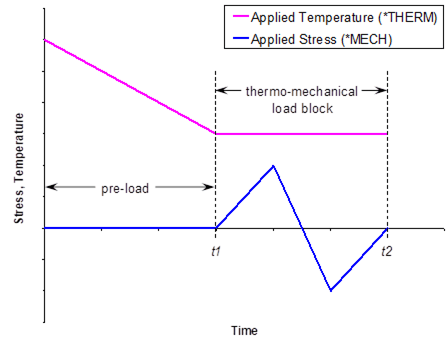
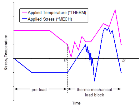
Figure 5.1 The MAC/GMC 4.0 fatigue damage analysis requires the specification of a thermo-mechanical “load block”, which defines a cycle of applied loading in the fatigue damage simulation. The load block is chosen from the thermo-mechanical loading specified under *MECH and *THERM by specifying BLOCK=t1,t2. (a) Simple example; (b) More involved example.

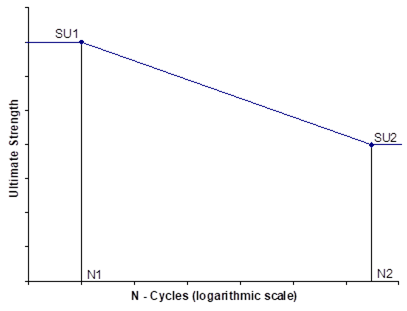
Figure 5.2 MAC/GMC 4.0 strength reduction fatigue damage model. Each component of the material’s ultimate strength is reduced according to the linear behavior defined by the points su1, su2, n1, and n2 from a semi-logarithmic plot.

*DEBOND: Fiber-matrix interfacial debonding

Purpose:

Enable interfacial debonding between the subcells within an RUC or laminate analysis. Two debonding models are available within MAC/GMC 4.0. Both models treat normal and shear interfacial debonding independently and incorporate finite shear and normal bond strengths. The constant compliant interface (CCI) model is formulated such that, after debonding occurs at a particular interface, the interfacial stress becomes a constant (for properly chosen model parameters). The evolving compliant interface (ECI) model, on the other hand, allows the interfacial stress to unload and be redistributed after debonding occurs (again, for properly chosen model parameters). While both models are made available, the ECI is thought to capture the physics of debonding better than the CCI model, especially when used in concert with HFGMC, which allows more accurate local stress redistribution than GMC. However, the CCI model may be useful in some instances in which one desires to maintain a certain amount of load carrying capacity subsequent to failure of the interface.

Usage:

*DEBOND

L=ly NII=nii

DBCH=dbch NAI=nai NBI=nbi NGI=ngi FACE=face BDN=s_DB LN=Λ_n BN=В_n TOLN=toln &

BDS=τ_DB LS=Λ_s BS=В_s DELAY=delay

® Repeated nii times

® Repeated nly times

Name	Definition
ly ¹	Layer number (Special Case)
nii	Number of debonding interfaces for layer ly
dbch	Debonding model choice = 1 ® Constant compliant interface (CCI) model = 2 ® Evolving compliant interface (ECI) model
nai ²	α index of subcell to which debonding model will be applied (see Figure 3.2) (Special Case)
nbi	β index of subcell to which debonding model will be applied (see Figure 3.1 and Figure 3.2)
ngi	γ index of subcell to which debonding model will be applied (see Figure 3.1 and Figure 3.2)
face	Interface to which debonding model will be applied (see Figure 5.3 and Figure 5.4)
s_DB ³	Normal interfacial bond strength
Λ_n ^3,4	ECI/CCI normal debonding parameter Λ
В_n ^3,4	ECI/CCI normal debonding parameter В
toln ^3,5	Reversal tolerance – stress below which interface is considered to be in compression
τ_DB ³	Shear interfacial bond strength
Λ_s ^3,4	ECI/CCI shear debonding parameter Λ
В_s ^3,4	ECI/CCI shear debonding parameter В
delay ⁶	Time delay – time before which interface is treated as perfectly bonded (sec.)

	face =	debonded face(s)
	1	Top face
	2	Right face
	3	Both faces

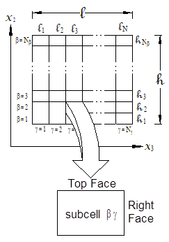
Figure 5.3 Definition of debonded faces for a given subcell within a doubly periodic RUC.

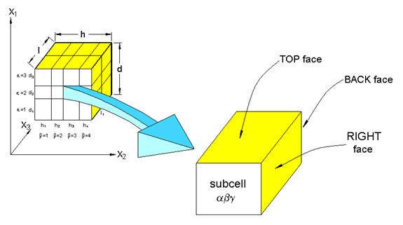
face =	debonded face(s)	face =	debonded face(s)
1	Top face	5	Top and Back faces
2	Right face	6	Right and Back faces
3	Back faces	7	All faces
4	Top and Right faces

Figure 5.4 Definition of debonded faces for a given subcell within a triply periodic RUC.

Examples:

*DEBOND

NII=2

DBCH=1 NBI=1 NGI=1 FACE=2 BDN=7. LN=0.0001 BN=60. TOLN=0. &

BDS=40 LS=0.1 BS=100. DELAY=64800.

DBCH=2 NBI=3 NGI=1 FACE=2 BDN=7. LN=0.0001 BN=8. TOLN=0. &

BDS=40 LS=0.1 BS=100 DELAY=64800.

*DEBOND

LY=1 NII=1

DBCH=1 NBI=1 NGI=1 FACE=2 BDN=10. LN=0.0001 BN=10. TOLN=0. &

BDS=40 LS=0.1 BS=100. DELAY=0.

LY=2 NII=0

LY=3 NII=1

DBCH=1 NBI=1 NGI=1 FACE=2 BDN=10. LN=0.0001 BN=10. TOLN=0. &

BDS=40 LS=0.1 BS=100. DELAY=0.

Associated MAC/GMC 4.0 Example Problem(s):

Example 5e

Notes:

1) L=ly is only required in the special case of laminate analysis. In this case, the debonding parameters for the interfaces in the RUCs representing each layer must be specified. If a layer has no debonding interfaces, LY=ly NII=0, should be specified (see Example above).

2) NAI=nai is only required in the special case of a triply periodic RUC. The triply periodic RUC may be part of a stand alone triply periodic RUC analysis or may represent a particular layer in a laminate analysis.

3) The units of s_DB, toln, and τ_DB must be consistent with the stress units employed throughout the analyzed problem. The units of В_n and В_s are seconds, while the units of Λ_n and Λ_s are 1/(stress units).

4) The debonding parameters, Λ_n, В_n, Λ_s, and В_s are constants in evolution equations that affect the debonding behavior of the interface. The form of these evolution equations is different for the CCI and CCI models. See the MAC/GMC 4.0 Theory Manual Section 5.4 for details on the debonding model equations.

5) The reversal tolerance, toln, can be used to force the interface to “close” when the normal stress is smaller than the specified value. The debonding model implementations within MAC/GMC 4.0 are such that, when the normal stress at a debonded interface becomes compressive, the interface “closes” and reacquires its original (perfectly bonded) normal stiffness. The reversal tolerance sets a small tensile value for the interfacial stress for the code to consider negligible.

6) The time delay, delay, can be used to artificially prevent debonding of the interface until after the specified time. This can be useful in situations where the user wished to disallow debonding during a portion of the applied loading history.

Additional Information:

MAC/GMC 4.0 Theory Manual Section 5.4

*CURTIN: Curtin effective fiber breakage model

Purpose:

Enable the Curtin effective fiber breakage model for subcells within a doubly periodic RUC (the model is not applicable to triply periodic RUCs). The Curtin model simulates the effects of fiber fracture and the unloaded portion of the fiber in the vicinity of the fiber fracture. The model uses statistical fiber strength data in order to simulate the effects of the breaking and subsequent load shedding of many fibers as one effective fiber. The effective fiber stiffness is degraded as the longitudinal stress in the fiber is increased. The effective longitudinal fiber stress reaches a maximum, which can be used as a failure stress for the effective fiber.

Usage:

*CURTIN

L=ly NCURT=ncurt

NBI=nbi NGI=ngi D=d L0=l₀ SIG0=s₀ TAU0=τ₀ M=m DELAY=delay ACTION=action

® Repeated ncurt times

® Repeated nly times

Name	Definition
ly ¹	Layer number (Special Case)
ncurt	Number of Curtin model effective fibers for layer ly
nbi	β index of subcell to which Curtin model will be applied (see Figure 3.1)
ngi	γ index of subcell to which Curtin model will be applied (see Figure 3.1)
d ²	Fiber diameter
l₀ ²	Fiber characteristic length
s₀ ³	Characteristic (average) fiber strength
τ₀ ^3,4	Shear stress sliding resistance at fiber-matrix interface
m	Weibull modulus from fiber strength statistics
delay ⁵	Time delay – time before which Curtin model is inactive
action	Action for code to take upon detection of Curtin model effective fiber failure: = 1 ® Zero fiber stiffness and continue execution = 0 ® Do nothing and continue (write notification to output file) = -1 ® Stop execution

Examples:

*CURTIN

NCURT=1

NBI=1 NGI=1 D=142.E-6 L0=0.0127 SIG0=508. TAU0=2.03 M=17.0 &

DELAY=64800. ACTION=0

*CURTIN

LY=1 NCURT=0

LY=2 NCURT=1

NBI=1 NGI=1 D=142.E-6 L0=0.0127 SIG0=610. TAU0=6.78 M=10.0 &

DELAY=0. ACTION=0

LY=3 NCURT=0

Associated MAC/GMC 4.0 Example Problem(s):

Example 5f

Notes:

1) L=ly is only required in the special case of laminate analysis. In this case, the Curtin model parameters for the fibers in the doubly periodic RUCs representing each layer must be specified. If a layer has no Curtin model fibers, LY=ly NCURT=0, should be specified.

2) The units for the fiber diameter and characteristic length, d and l₀, must have consistent (length) units, but these units do not have to be consistent with the remaining material property units.

3) The units of s₀ and τ₀ must be consistent with the stress units employed throughout the rest of the problem.

4) The shear stress sliding resistance at the fiber-matrix interface, τ₀, is the most difficult of the Curtin model parameters to obtain. Researchers have often attempted to deduce a value for this parameter from fiber push out and pull out tests on the composite. This parameter may also be chosen based on characterization vs. a known longitudinal composite stress-strain curve that is taken to failure.

5) The time delay, delay, can be used to artificially prevent activation of the Curtin model until after the specified time. This can be useful in situations where the user wishes to disallow fiber stiffness degradation and/or breakage during a portion of the applied loading history.

Additional Information:

MAC/GMC 4.0 Theory Manual Section 5.5

Section 6 : Results and Data Output Keywords

This section presents the four MAC/GMC 4.0 keywords that are related to the results of the analyzed problem. These are:

*PRINT ® Specify the level of results data to be written to the MAC/GMC 4.0 output file

*XYPLOT ® Specify data to be written to files for generating x-y scatter plots

*PATRAN ® Generate results output for post-processing with MSC/PATRAN software

*MATLAB ® Generate results output for post-processing with MATLAB software

The lowest level of data output in MAC/GMC 4.0 is controlled with the *PRINT keyword, which specifies the amount of data written to the ASCII format MAC/GMC 4.0 output file. Next, the *XYPLOT keyword writes time-based output to ASCII files that can be used within standard plotting software packages to generated x-y plots (such as predicted composite stress-strain curves). Finally, *PATRAN and *MATLAB enable the generation of data files to be read by the MSC/PATRAN and MATLAB (the MathWorks, Inc.) software packages for generating fringe plots that show the variation of the result fields over the composite architecture. Generation of fringe plots with these software packages requires the appropriate MAC/GMC 4.0 files (distributed with the MAC/GMC 4.0) that work in concert with *PATRAN and *MATLAB.

*PRINT: Overall print output level for output file

Purpose:

Specify the level of output data to be written to the MAC/GMC 4.0 ASCII output file

Usage:

*PRINT

NPL=npl

Name	Definition
npl	Print level specifier for the MAC/GMC 4.0 ASCII output file (see Table 6.1)

Table 6.1 Data written to the output file based on the value of npl.

*npl*	Result
-1	Determine and write effective properties and stop code execution
0	Minimal output, no effective properties, no time-based output
1	Time based global fields output, no effective properties
3	Effective RUC or laminate properties and architecture information
4	Debonding, yield surface, and static failure analysis information
6	Effective stiffness matrix and CTEs or ABD matrix output at each time step
7	Extensive fatigue damage information
8	Iteration data to screen for incremental plasticity and multimechanism GVIPS
9	Ancillary data
10	Program execution trace and all array data N Caution – Generates large output file and will slow execution considerably N

Example:

*PRINT

NPL=6

Associated MAC/GMC 4.0 Example Problem(s):

All example problems

Notes:

1) A print level of npl is inclusive of all output information associated with all print levels lower than npl.

2) If *PRINT is not specified, the code will use a default value of npl=1.

*XYPLOT: X-Y plot output

Purpose:

Generate time-based data for x-y scatter plots.

Usage:

*XYPLOT

FREQ=freq

LAMINATE=nlam

NAME=name_l X=x_l Y=y_l

® Repeated nlam times

MACRO=nmacro

NAME=name_mac LYR=lyr_mac X=x_mac Y=y_mac COORD=coord

® Repeated nmacro times

MICRO=nmicro

NAME=name_mic LYR=lyr_mic IA=ia IB=ib IG=ig X=x_mic Y=y_mic

® Repeated nmicro times

Name	Definition
freq	Frequency of time steps to write output (i.e., write output every freq time step)
nlam ¹	Number of laminate level plot files (Special Case)
name_l^1,2	Laminate level plot file name without path (Special Case)
x_l ¹	I.D. number of data to write in first column of data file for current laminate plot (see Table 6.2) (Special Case)
y_l ¹	I.D. number of data to write in second column of data file for current laminate plot (see Table 6.2) (Special Case)
nmacro	Number of macro (RUC level) plot files
name_mac²	Macro level plot file name without path
lyr_mac¹	Layer number for current macro plot (Special Case)
x_mac ³	I.D. number of data to write in first column of data file for current macro plot (see Table 6.3)
y_mac ³	I.D. number of data to write in second column of data file for current macro plot (see Table 6.3)

Name	Definition
coord ^1,4	Specifies local (principal material) or global (laminate) coordinate system for macro (RUC level) plots within laminate layer (Special Case) (Optional): = L ® Local coordinate system for layer (default if COORD=coord is omitted) = G ® Global (laminate) coordinate system
nmicro	Number of micro (subcell level) plot files
name_mac²	Micro level plot file name without path
lyr_mic¹	Layer number for current micro plot (Special Case)
ia ⁵	α subcell index for current micro plot (see Figure 3.2) (Special Case)
ib	β subcell index for current micro plot (see Figure 3.1 and Figure 3.2)
ig	γ subcell index for current micro plot (see Figure 3.1 and Figure 3.2)
x_mic ³	I.D. number of data to write in first column of data file for current micro plot (see Table 6.4)
y_mic ³	I.D. number of data to write in second column of data file for current micro plot (see Table 6.4)

Examples:

*XYPLOT

FREQ=5

MACRO=1

NAME=example_3a X=2 Y=8

MICRO=0

*XYPLOT

FREQ=1

LAMINATE=1

NAME=kxy_v_Mxy X=9 Y=15

MACRO=2

NAME=my_plot_file LYR=1 X=2 Y=8 COORD=G

NAME=” LYR=3 X=2 Y=14

MICRO=1

NAME=micro_file LYR=2 IB=1 IG=1 X=2 Y=8

Associated MAC/GMC 4.0 Example Problem(s):

Example 1c, Example 2a-h, Example 3a-i, Example 4a-d, Example 4h, Example 5b, Example 5d-f, Example 6a, Example 6b-c, Example 7a-c

Notes:

1) The x-y plot information associated with laminate level plots should only be specified in the special case of laminate analysis. Further, the specification of LYR=lyr_mac, LYR=lyr_mic, and COORD=coord for the macro and micro plots is only required in the special case of a laminate in order to indicate which layer the RUC or subcell information should be taken from.

2) Laminate level plot files have “_lam.data” appended to the specified name_l. Macro level plot files have “_macro.data” appended to the specified name_mac. Micro level plot files have “_micro.data” appended to the specified name_mic. The files will be written in the same directory as the input file. If a name is repeated within a particular level of plots, an integer counter will be appended to the specified file name. Finally, the special character double quotation (“) can be specified as a file name to automatically repeat the file name directly preceeding this specification (see Example above).

3) The macro and micro plot files associated with a laminate contain four columns of data rather than two. The first two columns contain the x and y data for quadrature point number 1 in the specified layer, while the third and fourth columns contain the x and y data for quadrature point number 2 in the specified layer.

4) Even in the case of laminate analysis, COORD=coord is optional. If it is omitted, the macro plot information will be written in the local coordinates of the layer.

5) IA=ia is only required in the special case when the subcell in question is part of a triply periodic RUC.

Table 6.2 LAMINATE level x-y plot data file i.d. numbers.

1		midplane normal strain	32	magnetic field
2		midplane normal strain	33	magnetic field
3		average normal strain	34	magnetic field
4		average engineering shear strain	35	electric force resultant
5		average engineering shear strain	36	electric force resultant
6		midplane engineering shear strain	37	electric force resultant
7		midplane curvature	38	electric moment resultant
8		midplane curvature	39	electric moment resultant
9		midplane curvature	40	electric moment resultant
10		force resultant	41	magnetic force resultant
11		force resultant	42	magnetic force resultant
12		force resultant	43	magnetic force resultant
13		moment resultant	44	magnetic moment resultant
14		moment resultant	45	magnetic moment resultant
15		moment resultant	46	magnetic moment resultant
16		inelastic force resultant	47	pyroelectric force resultant
17		inelastic force resultant	48	pyroelectric force resultant
18		inelastic force resultant	49	pyroelectric force resultant
19		inelastic moment resultant	50	pyroelectric moment resultant
20		inelastic moment resultant	51	pyroelectric moment resultant
21		inelastic moment resultant	52	pyroelectric moment resultant
22		thermal force resultant	53	pyromagnetic force resultant
23		thermal force resultant	54	pyromagnetic force resultant
24		thermal force resultant	55	pyromagnetic force resultant
25		thermal moment resultant	56	pyromagnetic moment resultant
26		thermal moment resultant	57	pyromagnetic moment resultant
27		thermal moment resultant	58	pyromagnetic moment resultant
28	N/A	N/A	59 - 99	N/A
29		electric field	100	temperature
30		electric field	101	time
31		electric field	102	creep time

Table 6.3 MACRO level x-y plot data i.d. numbers.

1		total normal strain	38	electric field
2		total normal strain	39	electric field
3		total normal strain	40	electric field
4		total engineering shear strain	41	magnetic field
5		total engineering shear strain	42	magnetic field
6		total engineering shear strain	43	magnetic field
7		stress	44	electric displacement
8		stress	45	electric displacement
9		stress	46	electric displacement
10		stress	47	magnetic flux density
11		stress	48	magnetic flux density
12		stress	49	magnetic flux density
13		inelastic normal strain	50	thermal electric field
14		inelastic normal strain	51	thermal electric field
15		inelastic normal strain	52	thermal electric field
16		inelastic engr. shear strain	53	thermal magnetic field
17		inelastic engr. shear strain	54	thermal magnetic field
18		inelastic engr. shear strain	55	thermal magnetic field
19-30		N/A	56-99	N/A
31		thermal normal strain	100	temperature
32		thermal normal strain	101	time
33		thermal normal strain	102	creep time
34		thermal engineering shear strain
35		thermal engineering shear strain
36		thermal engineering shear strain
37	N/A	N/A

Table 6.4 MICRO level x-y plot data i.d. numbers.

1	total normal strain	34	thermal engineering shear strain
2	total normal strain	35	thermal engineering shear strain
3	total normal strain	36	thermal engineering shear strain
4	total engineering shear strain	37	normal debond parameter
5	total engineering shear strain	38	normal debond parameter
6	total engineering shear strain	39	normal debond parameter
7	stress	40	shear debond parameter
8	stress	41	shear debond parameter
9	stress	42	shear debond parameter
10	stress	43	electric field
11	stress	44	electric field
12	stress	45	electric field
13	inelastic normal strain	46	magnetic field
14	inelastic normal strain	47	magnetic field
15	inelastic normal strain	48	magnetic field
16	inelastic engr. shear strain	49	electric displacement
17	inelastic engr. shear strain	50	electric displacement
18	inelastic engr. shear strain	51	electric displacement
19	inelastic model state variable	52	magnetic flux density
20	inelastic model state variable	53	magnetic flux density
21	inelastic model state variable	54	magnetic flux density
22	inelastic model state variable	55	thermal electric field
23	inelastic model state variable	56	thermal electric field
24	inelastic model state variable	57	thermal electric field
25	inelastic model state variable	58	thermal magnetic field
26	inelastic model state variable	59	thermal magnetic field
27	inelastic model state variable	60	thermal magnetic field
28	inelastic model state variable	61-99	N/A
29	inelastic model state variable	100	temperature
30	inelastic model state variable	101	time
31	thermal normal strain	102	creep time
32	thermal normal strain
33	thermal normal strain

*PATRAN: PATRAN post-processing data output

Purpose:

Generate data output files for post-processing using the MSC/PATRAN software in conjunction with the MACPOST software. The MACPOST software is an add-on to the MSC/PATRAN software package that enables generation of x-y plots and fringe plots. The MACPOST software add-on is distributed with MAC/GMC 4.0 and has its own User Manual (Goldberg et al., 1999). The user is referred to the MACPOST User Manual for specific instructions on post-processing the data generated from MAC/GMC 4.0. Note that the MSC/PATRAN output is available only for doubly and triply periodic GMC RUC analyses.

Usage:

*PATRAN

TPRE=tpre STP=stp

Name	Definition
tpre	Preloading time before which MSC/PATRAN output data files are not written
stp ¹	Frequency for writing MSC/PATRAN output, output is written every stp time step

Example:

*PATRAN

TPRE=57600. STP=50

Associated MAC/GMC 4.0 Example Problem(s):

Example 6b

Notes:

1) A small value of stp will cause a great deal of data to be written and may slow execution considerably.

2) The *PATRAN keyword causes the generation of the following 14 data files, where outfile is the MAC/GMC 4.0 output file name:

outfile.macgeo	RUC geometry data
outfile.total_pat.data	Number of time steps and subcells
outfile.macro1_pat.data	RUC level strain data at each output time
outfile.macro2_pat.data	RUC level stress data at each output time
outfile.macro3_pat.data	RUC level inelastic strain data at each output time
outfile.macro4_pat.data	RUC level thermal strain, creep time, temperature, and stress invariant data at each output time
outfile.micro1_pat.data	Subcell level strain data at each output time
outfile.micro2_pat.data	Subcell level stress data at each output time
outfile.micro3_pat.data	Subcell level inelastic strain data at each output time
outfile.micro4_pat.data	Subcell level thermal strain, creep time, temperature, and stress invariant data at each output time
outfile.micro1_pat.contour	Subcell level strain data for fringe plots
outfile.micro2_pat.contour	Subcell level stress data for fringe plots
outfile.micro3_pat.contour	Subcell level inelastic strain data for fringe plots
outfile.micro4_pat.contour	Subcell level thermal strain, creep time, temperature, and stress invariant data for fringe plots

*MATLAB: MATLAB post-processing data output

Purpose:

Generate data output files for post-processing using the MATLAB software in conjunction with the MATLAB source files distributed with MAC/GMC 4.0. The MATLAB output is available only for doubly periodic RUC analysis and doubly periodic RUC layers within a laminate analysis.

Usage:

*MATLAB

N=ntimes TIMES=t(1),t(2),…,t(ntimes)

Name	Definition
ntimes	Number of times at which MATLAB output will be written
t(1-ntimes)	The times at which MATLAB output will be written

Example:

*MATLAB

N=3 TIMES=57600.,57700.,57800.

Associated MAC/GMC 4.0 Example Problem(s):

Example 3f, Example 6c

Notes:

1) The *MATLAB keyword causes the generation of the following 5 data files, where outfile is the MAC/GMC 4.0 output file name:

outfile_x2.dat	x₂ subcell coordinate geometry information
outfile_x3.dat	x₃ subcell coordinate geometry information
outfile_sig.dat	Subcell level stress data at each output time
outfile_eps.dat	Subcell level strain data at each output time
outfile_epsp.dat	Subcell level inelastic strain data at each output time

To be read by the three MATLAB source files (see Note 2 below), the leading “outfile_” must be stripped from the outfile_x2.dat and outfile_x3.dat files. The remaining three MATLAB data files must contain only the data for a single time, without the time itself included. Thus, the user must copy the desired data out of the outfile_sig.dat, outfile_eps.dat, and outfile_epsp.dat files and copy it into the corresponding file with the leading “outfile_” stripped from the name. The MATLAB source files can then correctly read these three data files and create the appropriate fringe plots.

2) The following MATLAB source files, which generate fringe plots from the data contained in the MAC/GMC 4.0 MATLAB output files, are distributed with MAC/GMC 4.0:

stress.m	Generates stress component and invariant fringe plots
strain.m	Generates strain component fringe plots
epsp.m	Generates inelastic strain component fringe plots

Each file contains an explanation and a section for user edits that control some of the characteristics of the fringe plots. These MATLAB source files are printed in the Appendix.

3) The fringe plots can be generated by placing the MATLAB source files and the MAC/GMC 4.0 MATLAB output files in the MATLAB working directory, and then executing the MATLAB source files by typing the file name at the MATLAB command line. For example, typing “stress” at the MATLAB command line would execute the stress.m program to generate the stress component fringe plots.

Section 7 : End of File Keyword

This section contains the keyword that is required at the end of every MAC/GMC 4.0 input file:

*END ® Indicate that the end of the MAC/GMC 4.0 input file has been reached

*END: End of input file

P *END is a required keyword P

Purpose:

Define the end of the MAC/GMC 4.0 input file.

Usage:

*END

Example:

*END

Associated MAC/GMC 4.0 Example Problem(s):

All example problems

Notes:

1) Lines present in the input file that are after the *END keyword will not be read by the code. The user can thus hold particular lines of input file data by placing them after this keyword at the end of the input file.

References

Aboudi, J. (1989) “Micromechanical Analysis of Composites by the Method of Cells” Applied Mechanics Reviews 42(7), 193-221.

Aboudi, J. (1991) Mechnics of Composite Materials: A Unified Micromechanical Approach. Elsevier, New York.

Aboudi, J. (1995) “Micromechanical Analysis of Thermoinelastic Multiphase Short-Fiber Composites” Composites Engineering 5, 839-850.

Aboudi, J. (2000) “Micromechanical Prediction of the Effective Behavior of Fully Coupled Electro-Magneto-Thermo-Elastic Multiphase Composites” NASA/CR–2000-209787.

Aboudi, J., Pindera, M.-J., and Arnold, S.M. (2001) “Linear Thermoelastic Higher-Order Theory for Periodic Multiphase Materials” Journal of Applied Mechanics 68(5), 697-707.

Aboudi, J., Pindera, M.-J., and Arnold, S.M. (2002) “Higher-Order Theory for Periodic Multiphase Materials with Inelastic Phases” International Journal of Plasticity, in press. See also NASA/TM–2002-211469.

Arnold, S.M. and Kruch, S. (1994) “Differential Continuum Damage Mechanics Models for Creep and Fatigue of Unidirectional Metal Matrix Composites” International Journal of Damage Mechanics 3(2), 170-191.

Bednarcyk, B.A. (2002) “An Inelastic Micro/Macro Theory for Hybrid Smart/Metal Composites” Composites: Part B, in press. See also NASA/CR–2002-208521.

Bednarcyk, B.A. and Pindera, M.-J. (2000) “Inelastic Response of a Woven Carbon/Copper Composite – Part II: Micromechanics Model” Journal of Composite Materials 34(4), 299-331.

Goldberg, R.K., Comiskey, M.D., and Bednarcyk, B.A. (1999) “Micromechanics Analysis Code Post-Processing (MACPOST) User Guide Version 1.0” NASA/TM–1999-209062.

Herakovich, C.T. (1998) Mechanics of Fibrous Composites. John Wiley & Sons, New York.

Jones, R.M. (1975) Mechanics of Composite Materials, Hemisphere Publishing Corp., New York.

Paley, M. and Aboudi, J. (1992) “Micromechanical Analysis of Composites by the Generalized Cells Model” Mechanics of Materials 14, 127-139.

Pindera, M.-J. and Bednarcyk, B.A. (1999) “An Efficient Implementation of the Generalized Method of Cells of Unidirectional, Multi-Phased Composites with Complex Microstructures” Composites: Part B 30(1), 87-105.

Appendix

This Appendix contains the following:

· User-Defined Constituent Material Constitutive Model File

· User-Defined Stiffness Matrix Determination File

· User-Defined Material Property Determination File

· Sample external material database file

· The three MATLAB source files for generating fringe plots

® stress.m, strain.m, and epsp.m

User-Defined Constituent Material Constitutive Model File

usrmat.F90

!#######################################################################

SUBROUTINE USRMAT(DSA, SA, PE, PV, D, LOCTISO, TIME, TSTEP, &

CTEMP, DTEMPR, NIO, NE, NV, NS, MN, DMGF, NSASIZE)

!=======================================================================

! Purpose: MAC/GMC 4.0 user-defined material constitutive model for

! determination of the inelastic strain and state variable

! increments

! This subroutine is called when one or more constituent

! materials are described by user-defined constitutive

! models, that is, when:

! CMOD = 99

! Reference: MAC/GMC 4.0 Keywords Manual Section 2, MAC/GMC 4.0

! Example Manual (Example 2g)

! Called From: FORMIN

! Subs Called: FATALERROR

!=======================================================================

! * On Entry *

! SA -- Vector of total (integrated) quantities (see below)

! PE(NE) -- Vector of elastic constants for material MN

! (where NE = # of elastic constants --> 9 MAX)

! PV(NV) -- Vector of viscoplastic constants for material MN

! (where NV = # of viscoplastic constants --> 19 MAX)

! D(3) -- Vector of direction cosines (for models 3, 7, & 9)

! LOCTISO -- Flag indicating if ANY material exhibits local

! transverse isotropy (and global anisotropy)

! = 0 - all materials are at most globally transversely

! isotropic (D not used)

! = 1 - at least one material is locally transversely

! isotropic (D used)

! TIME -- Current time

! TSTEP -- Current time step

! CTEMP -- Current temperature

! DTEMPR -- Time rate of change of temperature

! NIO -- Unit number of .out file

! NE -- # of elastic constants --> 9 MAX

! NV -- # of viscoplastic constants --> 19 MAX

! NS -- Current subcell number (this routine is called from within

! a subcell loop)

! MN -- Material number

! DMGF -- Damage factor - if damage is included the user

! should multiply material stiffness terms by DMGF

! when using such terms in his inelastic model.

! * Expected On Exit *

! DSA -- Vector of quantity increments (see below)

!=======================================================================

! NOTE: In this subroutine, [SA] and [DSA] contain the

! micro (subcell) quantities for the micromechanics model

! Arrangement of [DSA] & [SA] arrays:

! variable location

! +------------------------------------------------------------

! | total strain (1-6) (contains ENGINEERING shears)

! |------------------------------------------------------------

! | stress (7-12)

! |------------------------------------------------------------

! | inelastic strain (13-18) (contains ENGINEERING shears)

! |------------------------------------------------------------

! | 12 "slots" (19-30)

! | for state variables

! |------------------------------------------------------------

! | thermal strain (31-36) (contains ENGINEERING shears)

! |------------------------------------------------------------

! | Rn & Rt debond (37 - Rn, 11 face)

! | parameters (38 - Rn, 22 face)

! | (39 - Rn, 33 face)

! | (40 - Rt, 11 face)

! | (41 - Rt, 22 face)

! | (42 - Rt, 33 face)

! +------------------------------------------------------------

! NOTE: The user is responsible for providing the inelastic strain and

! state variable increments, DSA slots (13-30). The rest of DSA

! should not be disturbed

! NOTE: To use your own code within this subroutine, this subroutine

! must be compiled and linked with the MAC/GMC 4.0 library file

! mac4.lib

! ** IT IS THE USER'S RESPONSIBILITY TO ENSURE THAT THE USER'S CODE **

! ** FUNCTIONS PROPERLY AND THAT THE DESIRED CODE IS ACTUALLY BEING **

! ** EXECUTED **

!=======================================================================

IMPLICIT DOUBLE PRECISION (A - H, O - Z)

DIMENSION SS(6), S(6), R(6)

DIMENSION DSA(NSASIZE), SA(NSASIZE)

DIMENSION PV(NV), PE(NE), D(3)

LOGICAL LOCTISO

!=======================================================================

NEP = 9

NVP = 19

IF( NE .GT. NEP ) THEN

CALL FATALERROR(NIO)

WRITE(NIO, *) 'TO MANY ELASTIC PROPERTIES FOR MATERIAL # ', MN

WRITE(NIO, *) ' # USED = ', NE

WRITE(NIO, *) ' # ALLOCATED = ', NEP

STOP

ENDIF

IF( NV .GT. NVP ) THEN

CALL FATALERROR(NIO)

WRITE(NIO, *) 'TO MANY NON-LINEAR PROPERTIES FOR MATERIAL # ', &

WRITE(NIO, *) ' # USED = ', NV

WRITE(NIO, *) ' # ALLOCATED = ', NVP

STOP

ENDIF

!***********************************************************************

! BEGIN USER EDITS *

!***********************************************************************

! -- Consider placing your own message here to ensure that your code is

! being executed

IF (TIME .EQ. 0.D0) THEN

WRITE(NIO, *) '*** NOTE: Default USRMAT routine being executed ***'

WRITE(*, *) '*** NOTE: Default USRMAT routine being executed ***'

ENDIF

!-----------------------------------------------------------------------

! MATERIAL #1 -- Power Law Creep

!-----------------------------------------------------------------------

IF (MN .EQ. 1) THEN

! -- Creep material properties

CREEPCOEF = PV(1)

POWER = PV(2)

! -- Deviatoric stress [S] in the subcell

TRACE3 = (SA(7) + SA(8) + SA(9)) / 3.

S(1) = SA(7) - TRACE3

S(2) = SA(8) - TRACE3

S(3) = SA(9) - TRACE3

S(4) = SA(10)

S(5) = SA(11)

S(6) = SA(12)

! -- Effective Stress

SEFF = SQRT((SA(7) - SA(8))**2 + (SA(8) - SA(9))**2 + &

(SA(7) - SA(9))**2 + &

+ 6 * (SA(10)**2 + SA(11)**2 + SA(12)**2)) / SQRT(2.)

CREEP_F = CREEPCOEF * SEFF**POWER

IF (SEFF .GT. 0.D0) THEN

COEF = 3 * CREEP_F / (2 * SEFF)

ELSE

COEF = 0.D0

ENDIF

! -- Inelastic strain increments

DSA(13) = COEF * S(1) * TSTEP

DSA(14) = COEF * S(2) * TSTEP

DSA(15) = COEF * S(3) * TSTEP

DSA(16) = COEF * S(4) * TSTEP

DSA(17) = COEF * S(5) * TSTEP

DSA(18) = COEF * S(6) * TSTEP

!-----------------------------------------------------------------------

! MATERIAL #2 --> Bodner-Partom

!-----------------------------------------------------------------------

ELSEIF (MN .EQ. 2) THEN

! -- Copy appropriate viscoplastic material constants

IF( NV .LT. 6 ) THEN

CALL FATALERROR(NIO)

WRITE(NIO, *) ' NOT ENOUGH PV SPACE: NV =', NV

STOP

ENDIF

D0 = PV(1)

Z0 = PV(2)

Z1 = PV(3)

BM = PV(4)

AN = PV(5)

Q = PV(6)

! -- Copy stress from [SA] to [SS]

SS(1) = SA(7)

SS(2) = SA(8)

SS(3) = SA(9)

SS(4) = SA(10)

SS(5) = SA(11)

SS(6) = SA(12)

! -- Compute the deviatoric stress [S] in the subcell

TEMP = (SS(1) + SS(2) + SS(3)) / 3.0

S(1) = SS(1) - TEMP

S(2) = SS(2) - TEMP

S(3) = SS(3) - TEMP

S(4) = SS(4)

S(5) = SS(5)

S(6) = SS(6)

AJ2 = 0.5 * (S(1)**2 + S(2)**2 + S(3)**2) + S(4)**2 + S(5)**2 + &

S(6)**2

SQ3AJ = DSQRT( SS(1)**2 + SS(2)**2 + SS(3)**2 + 2 * (SS(4)**2 + &

SS(5)**2 + SS(6)**2) )

SQ2 = 1.414215

IF (SQ3AJ .EQ. 0.0) THEN

DO I = 1, 6

R(I) = 0

END DO

ELSE

R(1) = SS(1) / SQ3AJ

R(2) = SS(2) / SQ3AJ

R(3) = SS(3) / SQ3AJ

R(4) = SQ2 * SS(4) / SQ3AJ

R(5) = SQ2 * SS(5) / SQ3AJ

R(6) = SQ2 * SS(6) / SQ3AJ

ENDIF

! -- If D0=0 then assume elastic and zero-out [DSA(13-30)] (inelastic

! strain increments and internal variable increments), then return

IF (D0 .EQ. 0) THEN

DO JJ = 13, 30

DSA(JJ) = 0.0

END DO

RETURN

! -- Inelastic

ELSE

ZEF = Z0 + Q * SA(20) + (1 - Q) * (R(1) * SA(21) + R(2) * &

SA(22) + R(3) * SA(23) + R(4) * SA(24) + R(5) &

* SA(25) + R(6) * SA(26))

IF (AJ2 .EQ. 0.0) THEN

AL = 0.0

ELSE

ARG1 = ZEF**2.0 / (3.0 * AJ2)

IF (ARG1 .GT. 1E6) ARG1 = 1E6

CON = .5 * (AN + 1.0) / AN

ARG = CON * (ARG1)**AN

IF (ARG .GT. 50.0) ARG = 50.0

AL = D0 / (DEXP(ARG) * DSQRT(AJ2))

ENDIF

! -- Inelastic strain increments

DSA(13) = AL * S(1) * TSTEP

DSA(14) = AL * S(2) * TSTEP

DSA(15) = AL * S(3) * TSTEP

DSA(16) = 2 * AL * S(4) * TSTEP

DSA(17) = 2 * AL * S(5) * TSTEP

DSA(18) = 2 * AL * S(6) * TSTEP

! -- Plastic work increment

WPD = S(1) * DSA(13) + S(2) * DSA(14) + S(3) * DSA(15) + S(4) * &

DSA(16) + S(5) * DSA(17) + S(6) * DSA(18)

! -- State variable increments

DSA(19) = WPD

Z0M = BM / Z0

ZD = Z0M * (Z1 - ZEF) * WPD

DSA(20) = ZD

DSA(21) = ZD * R(1)

DSA(22) = ZD * R(2)

DSA(23) = ZD * R(3)

DSA(24) = ZD * R(4)

DSA(25) = ZD * R(5)

DSA(26) = ZD * R(6)

ENDIF

!***********************************************************************

! END USER EDITS *

!***********************************************************************

RETURN

END

! *** EOF ***

User-Defined Stiffness Matrix Determination File

usrformde.F90

!#######################################################################

SUBROUTINE USRFORMDE(NIO, MN, TIME, PEM, PVM, D, D_MODEL, NE, NV, &

NEP, NVP, NMTS, DNEW)

!=======================================================================

! Purpose: MAC/GMC 4.0 user-defined subroutine to allow formation of

! constituent material stiffness matrices based on a user

! constitutive model, which may use arbitrary material

! properties (used when ncmd = 99)

! This subroutine is called when one or more constituent

! materials are described by user-defined constitutive

! models (using the USRMAT subroutine), that is, when:

! CMOD = 99

! Reference: MAC/GMC 4.0 Keywords Manual Section 2, MAC/GMC 4.0

! Example Manual (Example 2g)

! Called From: GETCON

! Subs Called:

!=======================================================================

! ** On Entry **

! NIO -- Unit number of .out file

! MN -- Material number

! TIME -- Current time

! PEM(NE, MN) -- Vector of elastic constants for material # MN

! PVM(NV, MN) -- Vector of viscoplastic constants for material # MN

! D(3) -- Vector of direction cosines

! (required for material models 3, 7, 9, & 20)

! D_MODEL -- Flag indicating if material # MN exhibits local

! transverse isotropy with global anisotropy

! = .FALSE. - material is at most globally transversely

! isotropic (D not used)

! = .TRUE. - material is locally transversely

! isotropic (D used)

! NE -- # of elastic constants --> 9 MAX

! NV -- # of viscoplastic constants --> 19 MAX

! NEP -- Max # of elastic constants (to dimension arrays)

! NVP -- Max # of viscoplastic constants (to dimension arrays)

! NMTS -- Total number of materials

! ** Expected On Exit **

! DNEW(6, 6) -- Current elastic material stiffness matrix

!=======================================================================!

! NOTE: In the examples shown here, standard engineering material

! elastic constants (E, nu) are used. However, the user is

! free to employ any material elastic constants with his

! constitutive model (i.e., bulk modulus, etc.). Thus, the

! user must provide the equations to determine the stiffness

! components required by GMC from his elastic constants.

! NOTE: To use your own code within this subroutine, this subroutine

! must be compiled and linked with the MAC/GMC 4.0 library file

! mac4.lib

! ** IT IS THE USER'S RESPONSIBILITY TO ENSURE THAT THE USER'S CODE **

! ** FUNCTIONS PROPERLY AND THAT THE DESIRED CODE IS ACTUALLY BEING **

! ** EXECUTED **

!=======================================================================!

IMPLICIT DOUBLE PRECISION (A - H, O - Z)

DIMENSION DNEW(6, 6)

DIMENSION PEM(NEP, NMTS), PVM(NVP, NMTS)

DIMENSION D(3)

LOGICAL D_MODEL

!***********************************************************************

!* BEGIN USER EDITS *

!***********************************************************************

! -- Consider placing your own message here to ensure that your code is

! being executed

IF (TIME .EQ. 0.D0) THEN

WRITE(NIO, *) '*** NOTE: Default USRFORMDE routine being executed ***'

WRITE(NIO, *) ' Material number', MN

WRITE(*, *) '*** NOTE: Default USRFORMDE routine being executed ***'

WRITE(*, *) ' Material number', MN

ENDIF

! -- Obtain material properties from storage

E = PEM(1, MN)

FN = PEM(2, MN)

GA = E / (2. * (1. + FN))

! -- Zero the stiffness matrix

DO I = 1, 6

DO J = 1, 6

DNEW(I, J) = 0

END DO

! -- Determine the stiffness components

GT = 0.5 * E / (1 + FN)

FK = 0.25 * E / (0.5 * (1 - FN) - FN**2)

DNEW(1, 1) = E + 4.0 * FK * FN**2

DNEW(2, 1) = 2.0 * FK * FN

DNEW(3, 1) = 2.0 * FK * FN

DNEW(1, 2) = 2.0 * FK * FN

DNEW(2, 2) = FK + GT

DNEW(3, 2) = FK - GT

DNEW(1, 3) = 2.0 * FK * FN

DNEW(2, 3) = FK - GT

DNEW(3, 3) = FK + GT

DNEW(4, 4) = GT

DNEW(5, 5) = GA

DNEW(6, 6) = GA

!***********************************************************************

! END USER EDITS *

!***********************************************************************

RETURN

END

! *** EOF ***

User-Defined Material Property Determination File

usrfun.F90

!#######################################################################

SUBROUTINE USRFUN(NIO, MN, TIME, TSTEP, CTEMP, DTEMPR, SA, DSA, &

DOLD, PEM, PVM, D, D_MODEL, ALPA, ALPT, &

NE, NV, NMTS, NEP, NVP, NSASIZE, SU1, SU2, N1, N2, &

ZDAM, NZDAM, XFAILT, XFAILC, NCRIT, CYCTOT)

!=======================================================================

! Purpose: MAC/GMC 4.0 user-defined subroutine to allow elastic and

! viscoplastic material properties to be functions of temp

! or field variables.

! This subroutine is called when one or more constituent

! materials employ user-defined functional form material

! properties, that is, when:

! (MATID .eq. 'U') .and. (MATDB = 2)

! Reference: MAC/GMC 4.0 Keywords Manual Section 2, MAC/GMC 4.0

! Example Manual (Example 2f)

! Called From: GETCON

! Subs Called:

!=======================================================================

! ** On Entry **

! NIO -- Unit number of MAC/GMC 4.0 output (.out) file

! MN -- Constituent material number

! TIME -- Current time

! TSTEP -- Current time step size

! CTEMP -- Current temperature

! DTEMPR -- Time rate of change of temperature

! SA -- Vector of total (integrated) quantities (see below)

! DSA -- Vector of quantity increments (see below)

! DOLD(6, 6) -- Previous elastic material stiffness matrix for material

! PEM(NE, MN) -- Vector of previous elastic constants for material

! # MN (where NE = # of elastic constants --> 9 MAX)

! PVM(NV, MN) -- Vector of previous viscoplastic constants for

! material # MN

! (where NV = # of viscoplastic constants --> 19 MAX)

! NMTS -- Total number of constituent materials

! NEP -- Max # of elastic constants (to dimension arrays)

! NVP -- Max # of viscoplastic constants (to dimension arrays)

! NSASIZE -- Length of the SA and DSA vectors (for dimensioning)

! NCRIT -- Number of failure criteria (for dimensioning)

! CYCTOT -- Current total number of cycles in damage analysis

! ** Expected On Exit **

! PEM(NE, MN) -- Vector of current elastic constants for material MN

! PVM(NV, MN) -- Vector of current viscoplastic constants for

! material MN

! D(3) -- Vector of direction cosines of normal to plane of

! trans. isotropy (required for models 3, 7, & 9)

! D_MODEL -- Flag indicating if material # MN exhibits local

! transverse isotropy with global anisotropy

! = .FALSE. - material is at most globally transversely

! isotropic (D not used)

! = .TRUE. - material is locally transversely

! isotropic (D used)

! ALPA(MN) -- Longitudinal cte for material MN

! ALPT(MN) -- Transverse cte for material MN

! NE -- Number of elastic properties used

! NV -- Number of viscoplastic properties used

! -------------- Strength reduction fatigue damage model ---------------

! SU1(MN, I) -- Material damage property (component I)

! SU2(MN, I) -- Material damage property (component I)

! N1(MN, I) -- Material damage property (component I)

! N2(MN, I) -- Material damage property (component I)

! -------------- Stiffness reduction fatigue damage model --------------

! ZDAM(MN,20) -- Material damage properties: (see manual)

! ZDAM(MN, 1) = ANG

! ZDAM(MN, 2) = BN

! ZDAM(MN, 3) = BP

! ZDAM(MN, 4) = OMU

! ZDAM(MN, 5) = OMFL

! ZDAM(MN, 6) = OMM

! ZDAM(MN, 7) = ETU

! ZDAM(MN, 8) = ETFL

! ZDAM(MN, 9) = ETM

! ZDAM(MN, 10) = BE

! ZDAM(MN, 11) = * empty *

! ZDAM(MN, 12) = A_hat

! ZDAM(MN, 13) = SFL

! ZDAM(MN, 14) = XML

! ZDAM(MN, 15) = SU

! ZDAM(MN, 16-20) = open space

! NZDAM(MN) -- SK - Flag to skip damage calculations for material

! = 0 - Perform damage calculations

! = 1 - Skip damage calculations

! ------------------ Local (subcell) failure model -------------------

! XFAILT -- Tensile failure properties (Xij), material #MN,

! (MN,ICRIT,I) criterion #ICRIT, component #I

! XFAILC -- Compressive failure properties (XCij), material #MN,

! (MN,ICRIT,I) criterion #ICRIT, component #I

!=======================================================================

! NOTE: This routine can be used in conjunction with an internal

! material constitutive model, or a constitutive model input by

! the user in the USRMAT subroutine

! NOTE: In this subroutine, [SA] and [DSA] contain the

! micro (subcell) quantities for the micromechanics model

! Arrangement of [DSA] & [SA] arrays:

! variable location

! +------------------------------------------------------------

! | total strain (1-6) (contains ENGINEERING shears)

! |------------------------------------------------------------

! | stress (7-12)

! |------------------------------------------------------------

! | inelastic strain (13-18) (contains ENGINEERING shears)

! |------------------------------------------------------------

! | 12 "slots" (19-30)

! | for state variables

! |------------------------------------------------------------

! | thermal strain (31-36) (contains ENGINEERING shears)

! |------------------------------------------------------------

! | Rn & Rt debond (37 - Rn, 11 face)

! | parameters (38 - Rn, 22 face)

! | (39 - Rn, 33 face)

! | (40 - Rt, 11 face)

! | (41 - Rt, 22 face)

! | (42 - Rt, 33 face)

! +------------------------------------------------------------

! NOTE: quantities in [SA] and [DSA] are SUBCELL quantities - the

! values on entry are for the first subcell containing material

! # MN - the values on exit of this subroutine will be applied to

! ALL SUBCELLS containing material # MN. It is thus recommended

! that, if using the field variables, you assign the appropriate

! material # to ONE SUBCELL ONLY. Use of [SA] and [DSA] in this

! context in conjunction with bending in laminate theory will

! result in erroneous results as field variables become dependent

! on through-thickness position (while the material # does not).

! NOTE: To use your own code within this subroutine, this subroutine

! must be compiled and linked with the MAC/GMC 4.0 library file

! mac4.lib

! ** IT IS THE USER'S RESPONSIBILITY TO ENSURE THAT THE USER'S CODE **

! ** FUNCTIONS PROPERLY AND THAT THE DESIRED CODE IS ACTUALLY BEING **

! ** EXECUTED **

!=======================================================================

IMPLICIT DOUBLE PRECISION (A - H, O - Z)

DIMENSION DOLD(6, 6), D(3)

DIMENSION PEM(NEP, NMTS), PVM(NVP, NMTS)

DIMENSION ALPA(NMTS), ALPT(NMTS)

DIMENSION DSA(NSASIZE), SA(NSASIZE)

DIMENSION SU1(NMTS, 6),SU2(NMTS, 6)

DIMENSION N1(NMTS, 6),N2(NMTS, 6)

DIMENSION ZDAM(NMTS, 20), NZDAM(NMTS)

DIMENSION XFAILT(NMTS, NCRIT, 6), XFAILC(NMTS, NCRIT, 6)

LOGICAL D_MODEL

!=======================================================================

!***********************************************************************

! BEGIN USER EDITS *

!***********************************************************************

! -- Consider placing your own message here to ensure that your code is

! being executed

IF (TIME .EQ. 0.D0) THEN

WRITE(NIO, *) '*** NOTE: Default USRFUN routine being executed ***'

WRITE(NIO, *) ' material number', MN

WRITE(*, *) '*** NOTE: Default USRFUN routine being executed ***'

WRITE(*, *) ' Material number', MN

ENDIF

!-----------------------------------------------------------------------

! MATERIAL # 1: Elastic, E = function of strain & previous E

!-----------------------------------------------------------------------

IF (MN .EQ. 1) THEN

IF (SA(1) .GT. 0) THEN

EAOLD = PEM(1, MN)

EA = 700.E9 - EAOLD * SA(1) * 80.0

ELSE

EA = 700.E9

EAOLD = 700.E9

ENDIF

IF (EA .GT. EAOLD) THEN

WRITE(NIO, *) 'NON-PHYSICAL REGIME ENTERED'

STOP

ENDIF

EA = EA

ET = EA

FNA = 0.41

FNT = 0.41

GA = EA / (2.0 * (1.0 + FNA))

ALPA(MN) = 4.5E-6

ALPT(MN) = 4.5E-6

NE = 5

PEM(1, MN) = EA

PEM(2, MN) = ET

PEM(3, MN) = FNA

PEM(4, MN) = FNT

PEM(5, MN) = GA

EA = EA

ET = EA

FNA = 0.41

FNT = 0.41

GA = EA / (2.0 * (1.0 + FNA))

ALPA(MN) = 4.5E-6

ALPT(MN) = 4.5E-6

NE = 5

PEM(1, MN) = EA

PEM(2, MN) = ET

PEM(3, MN) = FNA

PEM(4, MN) = FNT

PEM(5, MN) = GA

!-----------------------------------------------------------------------

! MATERIAL # 2: Incremental plasticity with strain rate dependence

!-----------------------------------------------------------------------

ELSEIF (MN .EQ. 2) THEN

EA = 13161.

ET = EA

FNA = 0.26

FNT = 0.26

GA = EA / (2.0 * (1.0 + FNA))

ALPA(MN) = 9.00E-6

ALPT(MN) = 9.00E-6

NE = 5

PEM(1, MN) = EA

PEM(2, MN) = ET

PEM(3, MN) = FNA

PEM(4, MN) = FNT

PEM(5, MN) = GA

NP = 3

NV = 2 * NP + 1

STRAIN_RATE = 0.4714 * (DSQRT((DSA(1) - DSA(2))**2 + (DSA(1) - DSA(3))**2 + &

(DSA(2) - DSA(3))**2 + 1.5 * DSA(4)**2 + &

1.5 * DSA(5)**2 + 1.5 * DSA(6)**2)) / TSTEP

IF (STRAIN_RATE .GT. 1.E-2) STRAIN_RATE = 1.E-2

IF (STRAIN_RATE .LT. 1.E-7) THEN

SY = 70.

S1 = 80.

S2 = 84.

S3 = 87.

ELSE

SY = 70. + 3. * LOG(1.E7*STRAIN_RATE)

S1 = SY + 10. * SY / 70.

S2 = SY + 14. * SY / 70.

S3 = SY + 17. * SY / 70.

ENDIF

E1=0.01

E2=0.015

E3=0.2

PVM(1, MN) = SY

PVM(2, MN) = S1

PVM(3, MN) = S2

PVM(4, MN) = S3

PVM(5, MN) = E1

PVM(6, MN) = E2

PVM(7, MN) = E3

!-----------------------------------------------------------------------

! MATERIAL # 3: properties = linear function of temperature

! for use with user constitutive model (actually b-p)

!-----------------------------------------------------------------------

ELSEIF (MN .EQ. 3) THEN

IF (CTEMP .LT. 21.0) CTEMP = 21.0

IF (CTEMP .GT. 400.) CTEMP = 400.

! -- Elastic

E = 72.4E9 - 81.53E6 * (CTEMP - 21.)

FN = 0.33 + 7.916E-5 * (CTEMP - 21.)

ALP = 22.5E-6 + 3.958E-9 * (CTEMP - 21.)

NE = 5

PEM(1, MN) = E

PEM(2, MN) = E

PEM(3, MN) = FN

PEM(4, MN) = FN

PEM(5, MN) = E / (2. * (1. + FN))

ALPA(MN) = ALP

ALPT(MN) = ALP

! -- Viscoplastic (Bodner-Partom)

D0 = 1.E4

Z0 = 340.E6

Z1 = 435.E6

BM = 300.0

AN = 10.0 - 0.02493 * (CTEMP - 21.)

Q = 1.0

NV = 6

PVM(1, MN) = D0

PVM(2, MN) = Z0

PVM(3, MN) = Z1

PVM(4, MN) = BM

PVM(5, MN) = AN

PVM(6, MN) = Q

!-----------------------------------------------------------------------

! MATERIAL # 4: Fiber (NCMD = 6) with local failure = funct of temp

!-----------------------------------------------------------------------

ELSEIF (MN .EQ. 4) THEN

PEM(1, MN) = 58.E3

PEM(2, MN) = 58.E3

PEM(3, MN) = 0.25

PEM(4, MN) = 0.25

PEM(5, MN) = 23.2E3

ALPA(MN) = 3.5E-6

ALPT(MN) = 3.5E-6

! -- Note: *SUBCELL_FAILURE must be specified in the input file to

! enable local failure checking. Any failure properties

! specified here will replace those specified in the input file

XFAILT(MN, 1, 1) = 3500. - 1.8 * (CTEMP - 21.)

!-----------------------------------------------------------------------

! MATERIAL #5: Matrix (NCMD = 6) with damage

!-----------------------------------------------------------------------

ELSEIF (MN .EQ. 5) THEN

PEM(1, MN) = 12770.

PEM(2, MN) = 12770.

PEM(3, MN) = 0.32

PEM(4, MN) = 0.32

PEM(5, MN) = PEM(1, MN)/(2. * (1.+ PEM(3, MN)))

ALPA(MN) = 21.06E-6

ALPT(MN) = 21.06E-6

! -- Note: *DAMAGE must be specified in the input file to enable fatigue

! damage analysis. Any damage properties specified here will

! replace those specified in the input file

ZDAM(MN, 1) = 0.

ZDAM(MN, 2) = 0.

ZDAM(MN, 3) = 0.

ZDAM(MN, 4) = 1.

ZDAM(MN, 5) = 1.

ZDAM(MN, 6) = 1.

ZDAM(MN, 7) = 1.

ZDAM(MN, 8) = 1.

ZDAM(MN, 9) = 1.

ZDAM(MN, 10)= 2.27

ZDAM(MN, 11) = 0

ZDAM(MN, 12) = 0.2302

ZDAM(MN, 13) = 20.3

ZDAM(MN, 14) = 900.

ZDAM(MN, 15) = 128.

NZDAM(MN) = 0

ENDIF

!***********************************************************************

! END USER EDITS *

!***********************************************************************

RETURN

END

! *** EOF ***

Sample external material database file

sample_material_database.mat

Sample Material Database Provided with MAC/GMC 4.0

# ------- Bodner-Partom Model Material

MAT=copper

CMOD=1

EL=120.E9,120.E9,0.33,0.33,45.11E9,14.7E-6,14.7E-6 &

VI=1.E4,63.E6,250.E6,8.19,7.5,0.55

# ------- Isotropic, Elastic Materials

MAT=SCS-6

CMOD=6

NTP=5

TEM=21.0,316.0,427.0,538.0,860.0

EA=393.E9,382.E9,378.E9,374.E9,368.E9

ET=393.E9,382.E9,378.E9,374.E9,368.E9

NUA=0.25,0.25,0.25,0.25,0.25

NUT=0.25,0.25,0.25,0.25,0.25

GA=157.2E9,152.8E9,151.2E9,149.6E9,147.2E9

ALPA=3.56E-6,3.73E-6,3.91E-6,4.07E-6,4.57E-6

ALPT=3.56E-6,3.73E-6,3.91E-6,4.07E-6,4.57E-6

# ------- User constitutive model example

MAT=Al(6061-0)

CMOD=99

NPE=2 NPV=6

NTP=6

TEM=21.0,148.9,204.4,260.0,371.1,400.0

E1=72.5E9,69.4E9,65.8E9,58.5E9,41.5E9,41.5E9

E2=0.33,0.33,0.33,0.33,0.33,0.33

ALPA=22.5E-6,22.5E-6,22.5E-6,22.5E-6,22.5E-6,22.5E-6

ALPT=22.5E-6,22.5E-6,22.5E-6,22.5E-6,22.5E-6,22.5E-6

V1=1.E4, 1.E4, 1.E4, 1.E4, 1.E4, 1.E4

V2=100.E6,100.E6,100.E6,100.E6,100.E6,100.E6

V3=190.E6,190.E6,190.E6,190.E6,190.E6,190.E6

V4=70.0,70.0,70.0,70.0,70.0,70.0

V5=10.0,7.0,4.0,1.6,0.55,0.55

V6=0.4,0.4,0.4,0.4,0.4,0.4

MATLAB source files for generation of fringe plots

stress.m

%------------------------------------------------------------------%

% stress.m MATLAB source file %

%------------------------------------------------------------------%

% Distributed with MAC/GMC 4.0

% This program will generate fringe plots with the MATLAB software

% from the data written to ASCII files by MAC/GMC 4.0 using the

% *MATLAB option

% This program reads the file sig.dat, which contains 8 columns:

% S11 S22 S33 S23 S13 S12 Smean Seff

% NOTE: Smean = (S11 + S22 + S33) / 3.

% Seff = sqrt(3*sij*sij/2) (sij = deviatoric stresses)

% = [1/sqrt(2)] * sqrt[(S11 - S22)**2 + (S22 - S33)**2 +

% (S11 - S33)**2 + 6*(S23**2 + S13**2 + S12**2)]

% While the ASCII output files from MAC/GMC 4.0 contain data for

% all specified times (and integration points for laminate), the

% sig.dat file should contain just the stress field data for the

% one particular time (and integration point) at which the fringe

% plots will be made.

% In addition, this program reads the files x2.dat and x3.dat,

% which are also generated by MAC/GMC 4.0 to define the subcell

% grid. Note that this grid will differ between GMC and HFGMC.

%------------------------------------------------------------------%

% -- Clear workspace

clear;

%------------------------------------------------------------------

% USER OPTIONS

%------------------------------------------------------------------

% -- Select stress components to plot (1 - plot, 0 - don't plot)

ns11 = 1;

ns22 = 1;

ns33 = 1;

ns23 = 1;

ns13 = 1;

ns12 = 1;

nsm = 1;

nse = 1;

% -- Select subplot (all on one Fig.) or individual Figs.

% nsub = 1 --> subplot

% nsub = 0 --> individual Figs.

nsub = 0;

% -- Set scale_spec = 1 to specify scale high and low values for each

% component - set values below

scale_spec = 0;

if scale_spec > 0

s11_low = -200;

s11_high = 500;

s22_low = -200;

s22_high = 500;

s33_low = -200;

s33_high = 500;

s23_low = -200;

s23_high = 500;

s13_low = -200;

s13_high = 500;

s12_low = -200;

s12_high = 500;

sm_low = -200;

sm_high = 500;

se_low = -200;

se_high = 500;

end

% -- Set average = 1 to perform averaging of tractions across subcell

% boundaries. This reproduces the average sense imposition of the

% traction continuity conditions in HFGMC.

% -- Set average = 0 for no averaging. Use average = 0 for GMC.

average = 0;

% -- Set nint = number of integration points in HFGMC when average = 1

if average > 0

nint = 11;

end

% -- Note: To draw subcell boundaries, change "shading interp"

% to "shading faceted" (GMC only)

%------------------------------------------------------------------

% END USER OPTIONS

%------------------------------------------------------------------

% -- Load x1.dat and x2.dat files and determine their sizes

load x2.dat;

m = length(x2);

load x3.dat;

n = length(x3);

% -- Create grid

[X,Y] = meshgrid(x3,x2);

% -- Load sig.dat file

load sig.dat;

f=1;

for i=1:m;

for j=1:n;

sig11(i,j) = sig(f,1);

sig22(i,j) = sig(f,2);

sig33(i,j) = sig(f,3);

sig23(i,j) = sig(f,4);

sig13(i,j) = sig(f,5);

sig12(i,j) = sig(f,6);

sigmean(i,j) = sig(f,7);

sigeff(i,j) = sig(f,8);

f=f+1;

end

%------------------------------------------------------------------

% Section to average boundary tractions

%------------------------------------------------------------------

if average > 0

Nbeta =length(x2)/nint;

for j=1:n

for i=1:Nbeta-1;

sig22(nint*i,j) = 0.5*(sig22(nint*i,j) + sig22(nint*i+1,j));

sig22(nint*i+1,j) = sig22(nint*i,j);

sig23(nint*i,j) = 0.5*(sig23(nint*i,j) + sig23(nint*i+1,j));

sig23(nint*i+1,j) = sig23(nint*i,j);

end

Ngama = length(x3)/nint;

for i=1:m

for j=1:Ngama-1;

sig33(i,nint*j) = 0.5*(sig33(i,nint*j) + sig33(i,nint*j+1));

sig33(i,nint*j+1) = sig33(i,nint*j);

sig23(i,nint*j) = 0.5*(sig23(i,nint*j) + sig23(i,nint*j+1));

sig23(i,nint*j+1) = sig23(i,nint*j);

end

%------------------------------------------------------------------

if nsub > 0

num_plots = ns11 + ns22 + ns33 + ns23 + ns12 + ns13 + nsm + nse;

if num_plots == 1

n1 = 2;

n2 = 2;

elseif num_plots == 2

n1 = 2;

n2 = 2;

elseif num_plots == 3

n1 = 2;

n2 = 2;

elseif num_plots == 4

n1 = 2;

n2 = 2;

elseif num_plots == 5

n1 = 3;

n2 = 3;

elseif num_plots == 6

n1 = 3;

n2 = 3;

elseif num_plots == 7

n1 = 3;

n2 = 3;

elseif num_plots == 8

n1 = 3;

n2 = 3;

end

num = 0;

if nsub > 0

figure;

hold on;

end

%------------------------------------------------------------------

% -- S11 plot

%------------------------------------------------------------------

if ns11 > 0

num = num + 1;

if nsub > 0

subplot(n1,n2,num);

else

figure;

hold on;

end

colormap(jet);

pcolor(X,Y,sig11), shading interp;

axis image;

if scale_spec > 0

caxis([s11_low s11_high]);

end

colorbar;

title('\bf\fontsize{24}\sigma\fontsize{14}_1_1');

xlabel('\bfx_3');

ylabel('\bfx_2','rotation',0);

end

%------------------------------------------------------------------

% -- S22 plot

%------------------------------------------------------------------

if ns22 > 0

num = num + 1;

if nsub > 0

subplot(n1,n2,num);

else

figure;

hold on;

end

colormap(jet);

pcolor(X,Y,sig22), shading interp;

axis image;

if scale_spec > 0

caxis([s22_low s22_high]);

end

colorbar;

title('\bf\fontsize{24}\sigma\fontsize{14}_2_2');

xlabel('\bfx_3');

ylabel('\bfx_2','rotation',0);

end

%------------------------------------------------------------------

% -- S33 plot

%------------------------------------------------------------------

if ns33 > 0

num = num + 1;

if nsub > 0

subplot(n1,n2,num);

else

figure;

hold on;

end

colormap(jet);

pcolor(X,Y,sig33), shading interp;

axis image;

if scale_spec > 0

caxis([s33_low s33_high]);

end

colorbar;

title('\bf\fontsize{24}\sigma\fontsize{14}_3_3');

xlabel('\bfx_3');

ylabel('\bfx_2','rotation',0);

end

%------------------------------------------------------------------

% -- S23 plot

%------------------------------------------------------------------

if ns23 > 0

num = num + 1;

if nsub > 0

subplot(n1,n2,num);

else

figure;

hold on;

end

colormap(jet);

pcolor(X,Y,sig23), shading interp;

axis image;

if scale_spec > 0

caxis([s23_low s23_high]);

end

colorbar;

title('\bf\fontsize{24}\sigma\fontsize{14}_2_3');

xlabel('\bfx_3');

ylabel('\bfx_2','rotation',0);

end

%------------------------------------------------------------------

% -- S13 plot

%------------------------------------------------------------------

if ns13 > 0

num = num + 1;

if nsub > 0

subplot(n1,n2,num);

else

figure;

hold on;

end

colormap(jet);

pcolor(X,Y,sig13), shading interp;

axis image;

if scale_spec > 0

caxis([s13_low s13_high]);

end

colorbar;

title('\bf\fontsize{24}\sigma\fontsize{14}_1_3');

xlabel('\bfx_3');

ylabel('\bfx_2','rotation',0);

end

%------------------------------------------------------------------

% -- S12 plot

%------------------------------------------------------------------

if ns12 > 0

num = num + 1;

if nsub > 0

subplot(n1,n2,num);

else

figure;

hold on;

end

colormap(jet);

pcolor(X,Y,sig12), shading interp;

axis image;

if scale_spec > 0

caxis([s12_low s12_high]);

end

colorbar;

title('\bf\fontsize{24}\sigma\fontsize{14}_1_2');

xlabel('\bfx_3');

ylabel('\bfx_2','rotation',0);

end

%------------------------------------------------------------------

% -- Smean plot

%------------------------------------------------------------------

if nsm > 0

num = num + 1;

if nsub > 0

subplot(n1,n2,num);

else

figure;

hold on;

end

colormap(jet);

pcolor(X,Y,sigmean), shading interp;

axis image;

if scale_spec > 0

caxis([sm_low sm_high]);

end

colorbar;

title('\bf\fontsize{24}\sigma\fontsize{14}_m_e_a_n');

xlabel('\bfx_3');

ylabel('\bfx_2','rotation',0);

end

%------------------------------------------------------------------

% -- Seff plot

%------------------------------------------------------------------

if nse > 0

num = num + 1;

if nsub > 0

subplot(n1,n2,num);

else

figure;

hold on;

end

colormap(jet);

pcolor(X,Y,sigeff), shading interp;

axis image;

if scale_spec > 0

caxis([se_low se_high]);

end

colorbar;

title('\bf\fontsize{24}\sigma\fontsize{14}_e_f_f');

xlabel('\bfx_3');

ylabel('\bfx_2','rotation',0);

end

clear;

break

% -- End of file

strain.m

%------------------------------------------------------------------%

% strain.m MATLAB source file %

%------------------------------------------------------------------%

% Distributed with MAC/GMC 4.0

% This program will generate fringe plots with the MATLAB software

% from the data written to ASCII files by MAC/GMC 4.0 using the

% *MATLAB option

% This program reads the file epsp.dat, which contains 6 columns:

% e11 e22 e33 e23 e13 e12

% ** NOTE: shear strains are engineering shears **

% While the ASCII output files from MAC/GMC 4.0 contain data for

% all specified times (and integration points for laminate), the

% eps.dat file should contain just the strain field data for the

% one particular time (and integration point) at which the fringe

% plots will be made.

% In addition, this program reads the files x2.dat and x3.dat,

% which are also generated by MAC/GMC 4.0 to define the subcell

% grid. Note that this grid will differ between GMC and HFGMC.

%------------------------------------------------------------------%

% -- Clear workspace

clear;

%------------------------------------------------------------------

% USER OPTIONS

%------------------------------------------------------------------

% -- Select strain components to plot (1 - plot, 0 - don't plot)

ne11 = 1;

ne22 = 1;

ne33 = 1;

ne23 = 1;

ne13 = 1;

ne12 = 1;

% -- Select subplot (all on one Fig.) or individual Figs.

% nsub = 1 --> subplot

% nsub = 0 --> individual Figs.

nsub = 0

% -- Set scale_spec = 1 to specify scale high and low values for each

% component - set values below

scale_spec = 0;

if scale_spec > 0

e11_low = -0.020;

e11_high = 0.025;

e22_low = -0.020;

e22_high = 0.025;

e33_low = -0.020;

e33_high = 0.025;

e23_low = -0.020;

e23_high = 0.025;

e13_low = -0.020;

e13_high = 0.025;

e12_low = -0.020;

e12_high = 0.025;

end

% -- Note: To draw subcell boundaries, change "shading interp"

% to "shading faceted" (GMC only)

%------------------------------------------------------------------

% END USER OPTIONS

%------------------------------------------------------------------

% -- Load x1.dat and x2.dat files and determine their sizes

load x2.dat;

m = length(x2);

load x3.dat;

n = length(x3);

% -- Create grid

[X,Y] = meshgrid(x3,x2);

% Load eps.dat file

load eps.dat;

f=1;

for i=1:m;

for j=1:n;

eps11(i,j) = eps(f,1);

eps22(i,j) = eps(f,2);

eps33(i,j) = eps(f,3);

eps23(i,j) = eps(f,4);

eps13(i,j) = eps(f,5);

eps12(i,j) = eps(f,6);

f=f+1;

end

%------------------------------------------------------------------

if nsub > 0

num_plots = ne11 + ne22 + ne33 + ne23 + ne12 + ne13;

if num_plots == 1

n1 = 2;

n2 = 2;

elseif num_plots == 2

n1 = 2;

n2 = 2;

elseif num_plots == 3

n1 = 2;

n2 = 2;

elseif num_plots == 4

n1 = 2;

n2 = 2;

elseif num_plots == 5

n1 = 3;

n2 = 3;

elseif num_plots == 6

n1 = 3;

n2 = 3;

end

num = 0;

if nsub > 0

figure;

hold on;

end

%------------------------------------------------------------------

% -- e11 plot

%------------------------------------------------------------------

if ne11 > 0

num = num + 1;

if nsub > 0

subplot(n1,n2,num);

else

figure;

hold on;

end

colormap(jet);

pcolor(X,Y,eps11), shading interp;

axis image;

if scale_spec > 0

caxis([e11_low e11_high]);

end

colorbar;

title('\bf\fontsize{24}\epsilon\fontsize{14}_1_1');

xlabel('\bfx_3');

ylabel('\bfx_2','rotation',0);

end

%------------------------------------------------------------------

% -- e22 plot

%------------------------------------------------------------------

if ne22 > 0

num = num + 1;

if nsub > 0

subplot(n1,n2,num);

else

figure;

hold on;

end

colormap(jet);

pcolor(X,Y,eps22), shading interp;

axis image;

if scale_spec > 0

caxis([e22_low e22_high]);

end

colorbar;

title('\bf\fontsize{24}\epsilon\fontsize{14}_2_2');

xlabel('\bfx_3');

ylabel('\bfx_2','rotation',0);

end

%------------------------------------------------------------------

% -- ep33 plot

%------------------------------------------------------------------

if ne33 > 0

num = num + 1;

if nsub > 0

subplot(n1,n2,num);

else

figure;

hold on;

end

colormap(jet);

pcolor(X,Y,eps33), shading interp;

axis image;

if scale_spec > 0

caxis([e33_low e33_high]);

end

colorbar;

title('\bf\fontsize{24}\epsilon\fontsize{14}_3_3');

xlabel('\bfx_3');

ylabel('\bfx_2','rotation',0);

end

%------------------------------------------------------------------

% -- e23 plot

%------------------------------------------------------------------

if ne23 > 0

num = num + 1;

if nsub > 0

subplot(n1,n2,num);

else

figure;

hold on;

end

colormap(jet);

pcolor(X,Y,eps23), shading interp;

axis image;

if scale_spec > 0

caxis([e23_low e23_high]);

end

colorbar;

title('\bf\fontsize{24}\gamma\fontsize{14}_2_3');

xlabel('\bfx_3');

ylabel('\bfx_2','rotation',0);

end

%------------------------------------------------------------------

% -- e13 plot

%------------------------------------------------------------------

if ne13 > 0

num = num + 1;

if nsub > 0

subplot(n1,n2,num);

else

figure;

hold on;

end

colormap(jet);

pcolor(X,Y,eps13), shading interp;

axis image;

if scale_spec > 0

caxis([e13_low e13_high]);

end

colorbar;

title('\bf\fontsize{24}\gamma\fontsize{14}_1_3');

xlabel('\bfx_3');

ylabel('\bfx_2','rotation',0);

end

%------------------------------------------------------------------

% -- e12 plot

%------------------------------------------------------------------

if ne12 > 0

num = num + 1;

if nsub > 0

subplot(n1,n2,num);

else

figure;

hold on;

end

colormap(jet);

pcolor(X,Y,eps12), shading interp;

axis image;

if scale_spec > 0

caxis([e12_low e12_high]);

end

colorbar;

title('\bf\fontsize{24}\gamma\fontsize{14}_1_2');

xlabel('\bfx_3');

ylabel('\bfx_2','rotation',0);

end

clear;

break

% -- End of file

epsp.m

%------------------------------------------------------------------%

% epsp.m MATLAB source file %

%------------------------------------------------------------------%

% Distributed with MAC/GMC 4.0

% This program will generate fringe plots with the MATLAB software

% from the data written to ASCII files by MAC/GMC 4.0 using the

% *MATLAB option

% This program reads the file epsp.dat, which contains 8 columns:

% ep11 ep22 ep33 ep23 ep13 ep12 ep_eq matnum

% ** NOTE: inelastic shear strains are engineering shears **

% NOTE: In the case of incremental plasticity constit model,

% ep_eq is the integrated equivalent plastic strain increment

% where dep_eq = sqrt(2*deijp*deijp/3)

% For other constit models, ep_eq = sqrt(2*eijp*eijp/3)

% see Mendelson, A. (1968) Plasticity: Theory and Application.

% While the ASCII output files from MAC/GMC 4.0 contain data for

% all specified times (and integration points for laminate), the

% epsp.dat file should contain just the inelastic strain field data

% for the one particular time (and integration point) at which the

% fringe plots will be made.

% In addition, this program reads the files x2.dat and x3.dat,

% which are also generated by MAC/GMC 4.0 to define the subcell

% grid. Note that this grid will differ between GMC and HFGMC.

%------------------------------------------------------------------%

% -- Clear workspace

clear;

%------------------------------------------------------------------

% USER OPTIONS

%------------------------------------------------------------------

% -- Select inelastic strain components to plot (1 - plot, 0 - don't plot)

nep11 = 1;

nep22 = 1;

nep33 = 1;

nep23 = 1;

nep13 = 1;

nep12 = 1;

nepeq = 1;

nmatn = 1;

% -- Select subplot (all on one Fig.) or individual Figs.

% nsub = 1 --> subplot

% nsub = 0 --> individual Figs.

nsub = 0;

% -- Set scale_spec = 1 to specify scale high and low values for each

% component - set values below

scale_spec = 1;

if scale_spec > 0

ep11_low = -0.005;

ep11_high = 0.015;

ep22_low = -0.005;

ep22_high = 0.015;

ep33_low = -0.005;

ep33_high = 0.015;

ep23_low = -0.005;

ep23_high = 0.015;

ep13_low = -0.005;

ep13_high = 0.015;

ep12_low = -0.005;

ep12_high = 0.015;

epeq_low = 0.0;

epeq_high = 0.03;

matn_low = 0;

matn_high = 4;

end

% -- Note: To draw subcell boundaries, change "shading interp"

% to "shading faceted" (GMC only)

%------------------------------------------------------------------

% END USER OPTIONS

%------------------------------------------------------------------

% -- Load x1.dat and x2.dat files and determine their sizes

load x2.dat;

m = length(x2);

load x3.dat;

n = length(x3);

% -- Create grid

[X,Y] = meshgrid(x3,x2);

% Load epsp.dat file

load epsp.dat;

f=1;

for i=1:m;

for j=1:n;

eps11p(i,j) = epsp(f,1);

eps22p(i,j) = epsp(f,2);

eps33p(i,j) = epsp(f,3);

eps23p(i,j) = epsp(f,4);

eps13p(i,j) = epsp(f,5);

eps12p(i,j) = epsp(f,6);

epspq(i,j) = epsp(f,7);

matnum(i,j) = epsp(f,8);

f=f+1;

end

%------------------------------------------------------------------

if nsub > 0

num_plots = nep11 + nep22 + nep33 + nep23 + nep12 + nep13 + nepeq + nmatn;

if num_plots == 1

n1 = 2;

n2 = 2;

elseif num_plots == 2

n1 = 2;

n2 = 2;

elseif num_plots == 3

n1 = 2;

n2 = 2;

elseif num_plots == 4

n1 = 2;

n2 = 2;

elseif num_plots == 5

n1 = 3;

n2 = 3;

elseif num_plots == 6

n1 = 3;

n2 = 3;

elseif num_plots == 7

n1 = 3;

n2 = 3;

elseif num_plots == 8

n1 = 3;

n2 = 3;

end

num = 0;

if nsub > 0

figure;

hold on;

end

%------------------------------------------------------------------

% -- ep11 plot

%------------------------------------------------------------------

if nep11 > 0

num = num + 1;

if nsub > 0

subplot(n1,n2,num);

else

figure;

hold on;

end

colormap(jet);

pcolor(X,Y,eps11p), shading interp;

axis image;

if scale_spec > 0

caxis([ep11_low ep11_high]);

end

colorbar;

title('\bf\fontsize{24}\epsilon\fontsize{14}^p_1_1');

xlabel('\bfx_3');

ylabel('\bfx_2','rotation',0);

end

%------------------------------------------------------------------

% -- ep22 plot

%------------------------------------------------------------------

if nep22 > 0

num = num + 1;

if nsub > 0

subplot(n1,n2,num);

else

figure;

hold on;

end

colormap(jet);

pcolor(X,Y,eps22p), shading interp;

axis image;

if scale_spec > 0

caxis([ep22_low ep22_high]);

end

colorbar;

title('\bf\fontsize{24}\epsilon\fontsize{14}^p_2_2');

xlabel('\bfx_3');

ylabel('\bfx_2','rotation',0);

end

%------------------------------------------------------------------

% -- ep33 plot

%------------------------------------------------------------------

if nep33 > 0

num = num + 1;

if nsub > 0

subplot(n1,n2,num);

else

figure;

hold on;

end

colormap(jet);

pcolor(X,Y,eps33p), shading interp;

axis image;

if scale_spec > 0

caxis([ep33_low ep33_high]);

end

colorbar;

title('\bf\fontsize{24}\epsilon\fontsize{14}^p_3_3');

xlabel('\bfx_3');

ylabel('\bfx_2','rotation',0);

end

%------------------------------------------------------------------

% -- ep23 plot

%------------------------------------------------------------------

if nep23 > 0

num = num + 1;

if nsub > 0

subplot(n1,n2,num);

else

figure;

hold on;

end

colormap(jet);

pcolor(X,Y,eps23p), shading interp;

axis image;

if scale_spec > 0

caxis([ep23_low ep23_high]);

end

colorbar;

title('\bf\fontsize{24}\gamma\fontsize{14}^p_2_3');

xlabel('\bfx_3');

ylabel('\bfx_2','rotation',0);

end

%------------------------------------------------------------------

% -- ep13 plot

%------------------------------------------------------------------

if nep13 > 0

num = num + 1;

if nsub > 0

subplot(n1,n2,num);

else

figure;

hold on;

end

colormap(jet);

pcolor(X,Y,eps13p), shading interp;

axis image;

if scale_spec > 0

caxis([ep13_low ep13_high]);

end

colorbar;

title('\bf\fontsize{24}\gamma\fontsize{14}^p_1_3');

xlabel('\bfx_3');

ylabel('\bfx_2','rotation',0);

end

%------------------------------------------------------------------

% -- ep12 plot

%------------------------------------------------------------------

if nep12 > 0

num = num + 1;

if nsub > 0

subplot(n1,n2,num);

else

figure;

hold on;

end

colormap(jet);

pcolor(X,Y,eps12p), shading interp;

axis image;

if scale_spec > 0

caxis([ep12_low ep12_high]);

end

colorbar;

title('\bf\fontsize{24}\gamma\fontsize{14}^p_1_2');

xlabel('\bfx_3');

ylabel('\bfx_2','rotation',0);

end

%------------------------------------------------------------------

% -- ep_eq plot

%------------------------------------------------------------------

if nepeq > 0

num = num + 1;

if nsub > 0

subplot(n1,n2,num);

else

figure;

hold on;

end

colormap(jet);

pcolor(X,Y,epspq), shading interp;

axis image;

if scale_spec > 0

caxis([epeq_low epeq_high]);

end

colorbar;

title('\bf\fontsize{24}\epsilon\fontsize{14}^p_e_q');

xlabel('\bfx_3');

ylabel('\bfx_2','rotation',0);

end

%------------------------------------------------------------------

% -- matnum plot

%------------------------------------------------------------------

if nmatn > 0

num = num + 1;

if nsub > 0

subplot(n1,n2,num);

else

figure;

hold on;

end

colormap(jet);

pcolor(X,Y,matnum), shading interp;

axis image;

if scale_spec > 0

caxis([matn_low matn_high]);

end

colorbar;

title('\bf\fontsize{20}materials');

xlabel('\bfx_3');

ylabel('\bfx_2','rotation',0);

end

clear;

break

% -- End of file

Index

Keywords

*ALLOWABLES, 80

*CHECK, 13

*CONDUCTIVITY, 14

*CONSTITUENTS, 21

*CURTIN, 98

*DAMAGE, 88

*DEBOND, 94

*ELECTROMAG, 16

*END, 113

*FAILURE_CELL, 86

*FAILURE_SUBCELL, 83

*LAMINATE, 60

*MATLAB, 110

*MDBPATH, 19

*MECH, 66

*PATRAN, 108

*PRINT, 101

*RUC, 48

*SOLVER, 72

*SURF, 76

*THERM, 70

*XYPLOT, 102

A=, 49, 89, 90

ACTION=, 83, 84, 85, 86, 87, 98, 99

Adams-Bashforth, 74

ALF1=, 31, 33

ALF2=, 31, 33

ALF3=, 31, 33

ALF4=, 31, 33

ALF5=, 31, 33

ALF6=, 31, 33

all subcells, 80, 91

allowables, 1, 5, 79, 80, 81, 82, 83

ALPA=, 26, 29, 30, 34, 35, 41, 43, 129

ALPT=, 26, 29, 30, 34, 35, 41, 43, 129

aluminum, 39, 129

ANG=, 60, 61, 62, 63, 89, 90

ANGINC=, 76

anisotropic, 3, 5, 21, 30, 32

arbitrary loading, 17

ARCHID=, 11, 48, 49, 50, 51, 56, 58, 60, 61, 62, 63

architecture, 1, 2, 45, 48, 49, 50, 51, 57, 60, 61, 62, 100, 101

architecture library, 48, 49, 51, 61

array dimensions, 13

AS=, 41, 43

ASCII files, 3, 9, 10, 100, 101, 130, 136, 141

ASP=, 49, 50, 61

ASP1=, 49, 61

ASP2=, 49, 61

aspect ratio, 50, 51

average material, 80

B=, 49

BDN=, 94, 96

BDS=, 94, 96

BE=, 89, 90

BLOCK=, 89, 90, 92

BN=, 89, 90, 94, 96

Bodner-Partom, 3, 21, 24, 28, 39, 118, 127, 129

bond strength, 94

BP=, 89, 90

BS=, 94, 96

build, 10

C=, 49

C11=, 31, 32

C12=, 31, 32

C13=, 31, 32

C14=, 31, 32

C15=, 31, 32

C16=, 31, 32

C22=, 31, 32

C23=, 31, 32

C24=, 31, 32

C25=, 31, 32

C26=, 31, 32

C33=, 31, 32

C34=, 31, 32

C35=, 31, 32

C36=, 31, 32

C44=, 31, 32

C45=, 31, 33

C46=, 31, 33

C55=, 31, 33

C56=, 31, 33

C66=, 31, 33

characteristic length, 98, 99

characterization, 27, 28, 99

check input file, 12

CMOD=, 11, 16, 22, 24, 25, 26, 28, 29, 30, 31, 32, 33, 35, 36, 37, 39, 40, 41, 43, 129

coefficient of thermal expansion, 27, 32, 34, 42

Coffin-Manson Law, 88

command prompt, 7, 10

Compaq Visual Fortran, 9, 10

compile, 9, 10, 36, 38

COMPR=, 80, 81, 83, 84, 86, 87

concentration equations, 79

conductivity, 14, 27, 34, 36

consistency, 40

constant compliant interface (CCI) model, 94, 96

constitutive model, 2, 3, 5, 9, 16, 18, 21, 22, 23, 24, 25, 26, 28, 30, 33, 34, 36, 37, 38, 40, 44, 73, 116, 121, 124, 127, 129

controlling component, 77

controlling subcell, 88, 89

COORD=, 102, 103, 104

coordinate system, 103

copper, 39, 88, 129

creep time, 105, 106, 107, 109

cross shaped fiber, 50

Curtin model, 1, 4, 6, 79, 98, 99

cyclic, 79, 88, 91

D=, 22, 23, 26, 28, 29, 36, 41, 43, 44, 49, 56, 58, 59, 62, 63, 98, 99

damage, 1, 2, 6, 74, 79, 85, 87, 88, 89, 90, 91, 92, 93, 101, 116, 123, 124, 127, 128

damage increment, 88, 89, 91

damage parameter, 88, 89, 91

data output, 1, 100, 108, 110

DBCH=, 94, 96

debonded face, 95

debonding, 1, 2, 4, 6, 79, 91, 94, 96, 97, 107, 117, 124

debonding parameter, 94, 96, 99

debug, 10

DELAY=, 94, 96, 98, 99

design allowables, 80

DINC=, 89, 90

directory, 7, 8, 9, 10, 19, 104, 111

directory path, 8, 9, 19

dissipation rate, 76

DOS, 7, 10

DR=, 49, 61, 76

E1=, 33, 35, 126, 129

E11=, 80, 81

E12=, 80, 81

E13=, 80, 81

E2=, 33, 35, 126, 129

E22=, 80, 81

E23=, 80, 81

E33=, 80, 81

EA=, 26, 29, 30, 41, 43, 129

EC11=, 80, 81

EC22=, 80

EC33=, 80

effective constitutive equation, 64

effective properties, 11, 45, 101

EL=, 11, 26, 29, 30, 32, 33, 35, 39, 41, 43, 129

electric displacement, 66, 69, 106, 107

electric field, 66, 68, 69, 105, 106, 107

electromagnetic, 5, 12, 16, 17, 20, 41, 42, 43, 44, 45, 60, 61, 62, 63, 64, 65, 66, 69

electromagnetic specifier, 16, 17, 20, 44, 61, 63

electromagnetically active, 44, 61, 63, 69

EM=, 16, 17, 20, 41, 43, 44, 60, 61, 62, 63

embedded, 45

ending time, 71, 73

engineering shear strain, 64, 68, 82, 85, 87, 105, 106, 107

EPS=, 76

equivalent plastic strain, 76, 141

ERR=, 72, 73, 74, 75

errors, 73, 74

ES=, 41, 43

ES11=, 41, 43

ES12=, 41, 43

ES26=, 41, 43

ET=, 26, 29, 30, 41, 43, 129

ETFL=, 89, 90

ETM=, 89, 90

ETU=, 89, 90

evolution equations, 96

evolving compliant interface (ECI) model, 94

Example Problem Manual, 2, 3, 6, 7

executable file, 7, 9, 10, 36, 38

execution, 5, 8, 10, 12, 13, 16, 69, 75, 77, 84, 86, 88, 91, 98, 101, 108, 111

execution speed, 10

external material database, 1, 5, 9, 18, 19, 20, 22, 27, 32, 34, 37, 39, 40, 42, 115, 129

EXTMAT=, 39

F=, 11, 48, 49, 50, 51, 61, 63

FACE=, 94, 96

failure, 2, 5, 6, 79, 81, 83, 84, 85, 86, 87, 88, 91, 94, 98, 99, 101, 123, 124, 127

failure criteria, 5, 79, 83, 86, 123

failure parameters, 83, 84, 85, 86, 87

fatigue, 6, 74, 79, 85, 87, 88, 89, 90, 91, 92, 93, 101, 123, 124, 128

fatigue damage exponent, 90

fatigue limit, 90

FeCrAlY, 24

fiber breakage, 1, 4, 6, 79, 98, 99

fiber diameter, 50, 99

fiber fracture, 6, 98

fiber material, 51

fiber radius, 50

fiber strength, 6, 79, 98

fiber volume fraction, 51, 55

field variables, 38, 72, 73, 75, 123, 124, 125

first subcell, 80, 124

flag-type keywords, 12

force resultant, 66, 68, 76, 77, 105

FORTRAN, 9, 10

forward Euler, 65, 73, 77

Freed-Walker viscoplastic model, 3, 5, 21, 25, 28

FREQ=, 102, 103

fringe plots, 1, 4, 6, 100, 108, 109, 111, 115, 130, 136, 141

GA=, 26, 29, 30, 41, 43, 129

Gauss quadrature, 45, 47

Getting Started, 1, 6, 7

global equilibrium, 72, 73

graphite, 11

GVIPS, 3, 5, 21, 24, 25, 28, 73, 74, 101

H=, 49, 56, 58, 62, 63

HFGMC, 2, 3, 4, 5, 6, 45, 46, 50, 51, 57, 59, 60, 61, 62, 63, 73, 94, 130, 131, 136, 141

I=, 48, 49, 50, 51

IA=, 102, 104

IB=, 102, 103

IG=, 102, 103

incremental plasticity model, 3, 5, 36, 73, 74, 101, 141

indices, 46

ineffective length, 98

inelastic material property, 27, 28, 34

inelastic power, 76

inelastic strain rate, 76

inelasticity, 2

initial time step, 75

input file, 1, 3, 4, 6, 7, 8, 9, 10, 11, 12, 13, 18, 19, 20, 21, 26, 27, 32, 34, 37, 39, 40, 42, 44, 45, 48, 60, 61, 87, 104, 112, 113, 127, 128

integration, 1, 45, 64, 65, 72, 73, 74, 77, 130, 131, 136, 141

integration points, 45, 72, 73, 130, 131, 136, 141

interface, 1, 3, 4, 6, 50, 51, 52, 53, 61, 79, 91, 94, 96, 97, 98, 99

interface material, 51, 61

interface thickness, 50

intermediate times, 69

internal material database, 18, 22, 23, 27, 32, 34, 35, 37, 38, 39, 40, 42, 44, 71

IP=, 76

ISPX=, 76, 78

ISPY=, 76, 78

ISR=, 76

ISTM=, 74

ISTT=, 74

iteration, 73

ITMAX=, 72, 73

K=, 11, 26, 29, 33, 35, 36, 39

KA=, 26, 34, 36

KS=, 41, 43

KS11=, 41, 43

KS22=, 41, 43

ksi, 18, 24, 25, 88

KT=, 26, 34, 36

L=, 56, 58, 62, 63, 94, 96, 98, 99

L0=, 98, 99

Lamé constants, 36

laminate, 2, 3, 4, 5, 6, 12, 14, 16, 17, 18, 44, 45, 47, 48, 60, 61, 62, 63, 64, 65, 66, 68, 69, 70, 73, 74, 76, 77, 78, 79, 80, 88, 89, 94, 96, 99, 101, 102, 103, 104, 110, 125, 130, 136, 141

laminate analysis, 2, 3, 5, 14, 16, 17, 45, 48, 60, 65, 68, 69, 74, 80, 94, 96, 99, 103, 104, 110

laminate level plot, 102, 103

LAMINATE=, 102, 103

lamination theory, 2, 5, 45

layer, 2, 4, 5, 16, 17, 18, 45, 47, 60, 61, 62, 63, 77, 78, 94, 96, 98, 99, 103, 104

Legendre polynomial, 72, 73

library file, 7, 9, 10, 21, 36, 38, 117, 121, 125

linear elastic, 18, 80, 83

link, 9, 10, 36, 38

LL=, 49

LN=, 94, 96

load block, 89, 91, 92

load magnitude, 6, 66, 69, 76, 77

load shedding, 98

loading, 2, 4, 5, 12, 14, 16, 17, 18, 23, 35, 38, 40, 44, 45, 64, 65, 66, 68, 69, 70, 71, 73, 74, 75, 76, 77, 78, 79, 83, 86, 88, 89, 91, 92, 97, 99

loading components, 17, 64, 65, 77

loading cycle, 88

loading option, 2, 17, 64, 65, 66, 68

LOP=, 17, 66, 67

LS=, 94, 96

LY=, 60, 61, 62, 63, 96, 99

LYR=, 102, 103

M=, 11, 22, 26, 27, 29, 30, 31, 32, 33, 34, 35, 37, 39, 41, 42, 43, 48, 49, 50, 51, 59, 61, 63, 90, 98, 99

mac4.exe, 7, 10

mac4.lib, 9, 21, 36, 38, 117, 121, 125

MACPOST, 4, 7, 108, 114

MAG=, 66, 67, 68

magnetic field, 66, 68, 69, 105, 106, 107

magnetic flux density, 66, 69, 106, 107

magnetic permeability, 42, 43

magnetoelectric, 42, 43

MAT=, 39, 40, 80, 81, 83, 84, 89, 90, 129

MATDB=, 11, 26, 29, 30, 31, 32, 33, 35, 37, 38, 39, 41, 43

material assignment, 57, 62

material number, 22, 27, 31, 34, 37, 38, 39, 42, 50, 81, 83, 84, 89, 123, 125

material point, 45

material properties, 3, 5, 9, 14, 16, 18, 21, 22, 23, 24, 26, 27, 29, 30, 31, 32, 33, 34, 35, 36, 37, 38, 39, 40, 41, 42, 43, 44, 79, 83, 91, 118, 122, 123

material property database, 3, 24

MATID=, 11, 14, 16, 22, 26, 29, 30, 31, 32, 33, 35, 37, 39, 41, 43

MATLAB, 1, 4, 6, 7, 100, 110, 111, 115, 130, 136, 141

matrix material, 51

maximum strain, 4, 83, 84, 85, 87

maximum stress, 83, 84, 85, 87

MAXNB=, 89, 90

mean stress, 90, 91

mechanical loading, 1, 5, 12, 17, 64, 65, 66, 71, 74, 83, 86, 88, 89, 91, 92

memory allocation, 3, 4, 13

METHOD=, 72, 74

micro level plot, 103

micromechanics, 2, 5, 6, 45, 48, 60, 88, 116, 124

Microsoft NotePad, 9

Microsoft WordPad, 9

midplane curvature, 68, 105

midplane strain, 45, 65, 66, 68, 76

MINSTEP=, 74, 75

MMAX=, 76

MOD=, 11, 16, 48, 49, 50, 51, 56, 58, 60, 61, 62, 63, 89, 90

mode, 66, 68, 76

MODE=, 66, 67, 68, 76

moment resultant, 45, 65, 68, 105

monolithic material, 50, 51, 57, 59, 60, 61, 62, 63

MPa, 18, 24, 25, 69

MS=, 41, 43

MS11=, 41, 43

MS22=, 41, 43

multimechanism, 3, 5, 73, 74, 101

N=, 110

N1=, 89, 90

N2=, 89, 90

NAI=, 94, 96

NAME=, 19, 102, 103

NARloy Z, 5, 21, 25

NASA, 2, 114

NBI=, 94, 96, 98, 99

NDMAT=, 89, 90

NGI=, 94, 96, 98, 99

NII=, 94, 96

NINTEG=, 72, 73

NiTi, 25

NLEG=, 72, 73

NLY=, 60, 61, 62, 63

NMAT=, 80, 81, 83, 84

NMATS=, 11, 22, 26, 29, 30, 31, 32, 33, 35, 37, 39, 41, 43

non-isothermal, 21

NP=, 26, 28, 29, 36

NPL=, 11, 101

NPT=, 66, 67, 68, 70, 71, 72

NPV=, 33, 35, 129

NTEMP=, 11, 14

NTP=, 26, 29, 30, 31, 32, 33, 35, 41, 43, 129

NUA=, 26, 29, 30, 41, 43, 129

number of subcells, 2, 4, 45, 51, 59

NUT=, 26, 29, 30, 41, 43, 129

OMFL=, 89, 90

OMM=, 89, 90

OMU=, 89, 90

ONERA, 88

open cell, 51

OPT=, 49

OPTION=, 76, 77, 78

optional, 8, 19, 23, 36, 38, 40, 44, 69, 77, 104

order, 2, 6, 7, 9, 11, 13, 19, 21, 36, 38, 40, 44, 73, 74, 77, 80, 98, 103

out-of-plane, 45

output, 1, 4, 6, 7, 8, 9, 10, 11, 14, 24, 77, 78, 84, 86, 98, 100, 101, 102, 108, 109, 110, 111, 123, 130, 136, 141

output file, 1, 7, 8, 9, 11, 14, 24, 77, 78, 84, 86, 98, 100, 101, 108, 110, 111, 130, 136, 141

P100, 24

packing, 51

particulate, 5

PATH=, 19

PATRAN, 1, 4, 7, 100, 108

PDF, 7

PELS=, 41, 43

PELS1=, 42, 43

PELS2=, 42, 43

perfectly bonded, 94, 96

piezoelectric, 42

piezomagnetic, 42

plane of transverse isotropy, 22, 27, 42

plot file data i.d. number, 102, 103, 105, 106, 107

ply, 2, 4, 5, 16, 17, 18, 45, 47, 60, 61, 62, 63, 77, 78, 94, 96, 98, 99, 103, 104

PMGS=, 41, 43

PMGS1=, 42, 43

PMGS2=, 42, 43

Poisson ratio, 27, 42

post-processing, 1, 6, 7, 100, 108, 110

preload, 65, 77

print level, 101

probing, 65, 76, 77, 78

project, 9, 10

pyroelectric, 42, 43, 105

pyromagnetic, 42, 43, 105

QS=, 41, 43

QS11=, 41, 43

QS12=, 41, 43

QS26=, 41, 43

R=, 48, 49, 50, 51, 61

RA=, 49

RAD=, 48, 49

RAD1=, 49, 51

RAD2=, 49, 51

RC=, 49

RD=, 49

redistribution, 88, 89, 94

references, 7

REFTIME=, 66, 69

repeating unit cell analysis, 14, 16, 45, 48, 51, 59, 60, 61, 63, 64, 65, 69, 73, 78, 80, 96, 110

repeating unit cell dimensions, 50

repeating unit cell failure, 86

residual stresses, 69, 77, 79

results, 2, 6, 7, 8, 9, 10, 13, 36, 38, 73, 75, 100, 125

reversal tolerance, 96

RITFR=, 48, 49, 50

RITFR1=, 49, 51

RITFR2=, 49, 51

RL=, 49

RLC=, 49

Robinson viscoplastic model, 3, 5, 21, 24, 25, 28

Runge-Kutta, 74

S11=, 80, 81

S12=, 80, 81

S13=, 80, 81

S22=, 80, 81

S23=, 80, 81

S33=, 80, 81

SC11=, 80

SC22=, 80

SC33=, 80

scatter, 100, 102

SCS-6, 24, 39, 129

self-adaptive, 65, 72, 74

semi-logarithmic, 88, 93

semi-major axis, 50

SFL=, 89, 90

shape memory alloy, 3, 5, 21

shear modulus, 27, 42

shear strength, 90

SiC, 24

SIG0=, 98, 99

slave component, 77, 78

sliding resistance, 98, 99

SM=, 56, 57, 58, 62, 63

smart, 2, 5, 12, 22, 41, 44

S-N curve, 88, 91

source, 1, 4, 6, 7, 9, 10, 36, 38, 110, 111, 115, 130, 136, 141

special case, 6, 21, 23, 35, 36, 38, 40, 44, 51, 59, 61, 63, 64, 65, 69, 73, 77, 82, 85, 87, 96, 99, 103, 104

special characters, 11

starting time, 71, 73

state variables, 9, 88, 107, 116, 117, 124

static failure, 1, 4, 5, 6, 79, 83, 86, 101

step size, 72, 73, 74, 75, 76, 77, 123

stiffness matrix, 36, 64, 101, 121, 122, 123

stiffness reduction, 6, 79, 88, 91

STP=, 72, 76, 108

strain allowables, 80, 81, 82, 87

strain reference time, 66

strength reduction, 4, 6, 79, 88, 90, 93

stress allowables, 81

stress-strain curve, 5, 27, 28, 99, 100

SU=, 89, 90

SU1=, 89, 90

SU2=, 89, 90

subcell failure, 84

surf_1st.dat, 78

surf_1st_ply.dat, 78

surf_all.dat, 78

surf_all_plies.dat, 78

surf_global.dat, 78

surf_local.dat, 78

surf_plies.dat, 78

T300, 24

T50, 24

TAU0=, 98, 99

TEM=, 26, 29, 30, 31, 32, 33, 35, 41, 43, 129

TEMP=, 11, 14, 70, 71

temperature, 3, 9, 18, 22, 23, 25, 27, 31, 32, 34, 35, 36, 37, 38, 39, 40, 42, 43, 44, 45, 65, 70, 71, 76, 77, 91, 105, 106, 107, 109, 116, 123, 127

temperature points, 70

temperature unit, 18, 25, 71

temperature-dependent, 23, 35, 38, 40, 44, 91

temperature-independent, 3, 23, 36, 38, 40, 44

Theory Manual, 2, 7, 17, 21, 23, 30, 44, 45, 51, 59, 61, 63, 65, 69, 71, 74, 75, 78, 82, 85, 87, 91, 96, 97, 99

thermal loading, 1, 64, 70, 73, 74, 75, 91

THK=, 60, 61, 62, 63

through-thickness, 45, 125

TI=, 66, 67, 68, 70, 71, 72

Ti-15-3, 25

Ti-21S, 24, 25

Ti-24-11, 25

Ti-6-4, 24

time delay, 97, 99

time integration, 65, 72, 73, 77

time unit, 18

TIMES=, 110

titanium, 24, 25, 79

title, 10, 40, 133, 134, 135, 136, 138, 139, 140, 141, 143, 144, 145, 146

TMAX=, 76

TOLN=, 94, 96

TPRE=, 108

transversely isotropic, 3, 15, 16, 21, 36, 44, 91

TREF=, 22, 23, 26, 30, 31, 33, 35, 36, 37, 38, 39, 40, 41, 44, 76, 77

Tsai-Hill, 4, 83, 84, 85, 86, 87

ultimate strength, 90, 93

units, 18, 25, 50, 69, 71, 96, 99

user-defined, 3, 7, 9, 10, 14, 16, 18, 19, 22, 23, 27, 28, 32, 34, 35, 36, 37, 38, 39, 40, 42, 44, 50, 57, 58, 60, 62, 116, 121, 123

usrformde, 1, 9, 21, 36, 121

usrfun, 1, 3, 9, 27, 32, 34, 37, 38, 39, 42, 123

usrmat, 1, 3, 9, 21, 36, 38, 116, 141

V1=, 26, 29, 30, 34, 35, 129

V2=, 26, 29, 30, 34, 35, 129

VF=, 11, 48, 49, 50, 61, 63

VF1=, 49, 51

VI=, 26, 29, 33, 35, 36, 39, 129

volume fraction, 50, 51, 55

Weibull modulus, 98

Windows, 7, 9

workspace, 130, 136, 141

X=, 102, 103

X11=, 83, 84, 86, 87

X12=, 83, 84, 86, 87

X13=, 83, 84, 86, 87

X22=, 83, 84, 86, 87

X23=, 83, 84, 86, 87

X33=, 83, 84, 86, 87

XA=, 48

XC11=, 83, 86

XC22=, 83, 84, 86, 87

XC33=, 83, 84, 86, 87

XML=, 89, 90

x-y plot, 4, 100, 103, 105, 106, 107, 108

Y=, 102, 103

yield criteria, 77

yield surface, 2, 5, 27, 28, 64, 65, 73, 76, 77, 78, 101

zero stiffness, 88, 91